The starting point for the development of dashed line theory was a particular way to observe the sequence of prime numbers:
If we add 2 (the first prime number) to all the sequence elements, we’ll obtain
If we add three (the second prime number) we’ll obtain
Going on this way, and reordering the results, the following table is obtained, in which every column contains the value of the sum, every row contains the first addend, and their intersection contains the second one:
| first addend \ sum | 2 | 3 | 4 | 5 | 6 | 7 | 8 | 9 | 10 | 11 | 12 | 13 | 14 | 15 | 16 | 17 | 18 | 19 | 20 |
|---|---|---|---|---|---|---|---|---|---|---|---|---|---|---|---|---|---|---|---|
| 2+ | 2 | 3 | 5 | 7 | 11 | 13 | 17 | ||||||||||||
| 3+ | 2 | 3 | 5 | 7 | 11 | 13 | 17 | ||||||||||||
| 5+ | 2 | 3 | 5 | 7 | 11 | 13 | |||||||||||||
| 7+ | 2 | 3 | 5 | 7 | 11 | 13 | |||||||||||||
| 11+ | 2 | 3 | 5 | 7 | |||||||||||||||
| … | … | … | … | … | … | … | … | … | … | … | … | … | … | … | … | … | … | … | … |
In reference to Table 1, the Goldbach’s conjecture states that the columns corresponding to even numbers, from 4 on, are never empty.
It’s clear that such a property originates from the “dovetailing” of the sequence of prime numbers with itself, with “offsets” that are the prime numbers themselves and that we indicated with “2+”, “3+”, “5+”, etcetera. How to prove that in this complex interlocking game no “holes”, that are empty columns, are left, at least in correspondence with even numbers greater than 2? To Simone’s knowledge, a mathematical theory allowing to explain in detail what happens in such tables, concerning possible dovetails and empty columns, didn’t exist. In order to respond to this lack, he began to develop the dashed line theory.
Non only the sums of primes, but also prime numbers themselves can be described with tables similar to Table 1. For example we can consider the following table:
| 0 | 1 | 2 | 3 | 4 | 5 | 6 | 7 | 8 | 9 | 10 | 11 | 12 | 13 | 14 | 15 | 16 | 17 | 18 | 19 | 20 |
|---|---|---|---|---|---|---|---|---|---|---|---|---|---|---|---|---|---|---|---|---|
| 0 | 2 | 4 | 6 | 8 | 10 | 12 | 14 | 16 | 18 | 20 | ||||||||||
| 0 | 3 | 6 | 9 | 12 | 15 | 18 | ||||||||||||||
| 0 | 4 | 8 | 12 | 16 | 20 | |||||||||||||||
| 0 | 5 | 10 | 15 | 20 |
The differences with respect to Table 1 are the following:
- The sequence of integers in the rows isn’t always the same: the sequence in the first row is (2x)_{x \geq 0} = 0, 2, 4, 6, 8, \dots, the one in the second row is (3x)_{x \geq 0} = 0, 3, 6, 9, 12, \dots, and so on. In general, the sequence of integers in the i-th row is ((i+1)x)_{x \geq 0};
- There isn’t an initial “offset” that changes among rows: in all rows the sequence starts with the number 0 in column number 0.
In other terms, while in Table 1 the sequence of the integers in each row is always the same (the sequence of prime numbers), but each row has a different offset with respect to the first row (a prime number), in Table 2 each row has a different sequence, but all the sequences have the number 0 in column 0, so they are, in this sense, “synchronized”.
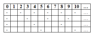
A consequence of this “synchronization” is that the numbers in the cells always coincide with the number of the column in which they appear, so they don’t convey any additional information, apart from being (cell containing a number) or not (empty cell). Therefore they can be replaced by a simple dash, thus simplifying the table without losing any information:
| 0 | 1 | 2 | 3 | 4 | 5 | 6 | 7 | 8 | 9 | 10 | 11 | 12 | 13 | 14 | 15 | 16 | 17 | 18 | 19 | 20 |
|---|---|---|---|---|---|---|---|---|---|---|---|---|---|---|---|---|---|---|---|---|
| – | – | – | – | – | – | – | – | – | – | – | ||||||||||
| – | – | – | – | – | – | – | ||||||||||||||
| – | – | – | – | – | – | |||||||||||||||
| – | – | – | – | – |
The interesting aspect, as we mentioned before, is that prime numbers can be described by tables of this kind. In fact, looking at Table 3, we immediately know if a given number n is divisible by 2, or by 3, or by 4 or 5: it’s sufficient to see what dashed are present in column n. This information helps in identifying prime numbers, as we’ll specify in a while in the paragrafh Dashed lines and prime numbers.
Table 3 is a graphical representation of an object that we’ll call dashed line, for how table rows appear. More precisely, in this case it’s a linear dashed line, because the sequence of the column numbers of the dashes in each row is linear, and in particular of the kind
for some fixed positive integer n (in the example, n = 2, 3, 4, 5). As this number n varies from one row to the other, it’s convenient to denote it with n_i, where i varies from 1 to the number of table rows. Thus we’ll indicate with n_1 the number n associated to the first row, with n_2 the number n associated to the second row, etcetera, so in Table 3 we have that n_1, n_2, n_3, n_4 are respectively 2, 3, 4, 5. Therefore the sequence in row i becomes
Of course each of these sequences is infinite, so, ideally, Table 3 should also have infinite columns (still starting from 0). Indeed, according to the context, just a portion of the table, the one that’s needed for illustrating the concepts to be expressed, is displayed, but it’s implied that the table should have infinite columns.
Given the mathematical law (2), a table like Table 3 is completely determined by the constants n_1, n_2, \dots, n_k, where k is the number of table rows. These constants are called components of the dashed line; in particular n_1 is the component associated to the first row, n_2 is the component associated to the second row, …, in general n_i is the component associated to row i. By extension, we’ll say also dashes of row i to have component n_i. We’ll also indicate the dashed line with the k-tuple (n_1, n_2, \dots, n_k). So Table 3 is the graphical representation of the dashed line (2, 3, 4, 5). We shall see later, in the post Dashed lines, dashes and spaces: some definitions and simple properties, the mathematical definition of dashed line, but it’s not important for now: it’s enough to know that the dashed line (2, 3, 4, 5) is the equivalent, in mathematical instead of graphical terms, of Table 3.
Having chosen a linear sequence like (2), for deciding where to place the dashed of row i, there are two consequences:
- Dashes of the same row are equidistant to each other, and their distance is equal to the component associated to the row;
- Column 0 contains a dash for each row.
An important thing to note is that, in tables like Table 3, the general arrangement of the dashes repeats itself every M columns, where M is the least common multiple of the dashed line components. For example, in Table 3, M = \mathrm{MCM}(2, 3, 4, 5) = 60. In fact 60, being the least common multiple of the components, is divisible by each of them, like 0. So column 60 will contain a dash for each row, just like column 0. From that column on, it’s easy to see (and, if you want, to prove) that the outline of the dashed line repeats itself identically: column 61 contains the same number of dashes, in the same rows, of column 1, and the same thing happens for the other columns, as you can see by comparing column 62 with column 2, 63 with column 3, and so on:
| 0 | 1 | 2 | 3 | 4 | 5 | 6 | 7 | 8 | 9 | 10 | 11 | 12 | 13 | 14 | 15 | 16 | 17 | 18 | 19 | 20 | \dots | 60 | 61 | 62 | 63 | 64 | 65 | \dots |
|---|---|---|---|---|---|---|---|---|---|---|---|---|---|---|---|---|---|---|---|---|---|---|---|---|---|---|---|---|
| – | – | – | – | – | – | – | – | – | – | – | \dots | – | – | – | \dots | |||||||||||||
| – | – | – | – | – | – | – | \dots | – | – | \dots | ||||||||||||||||||
| – | – | – | – | – | – | \dots | – | – | \dots | |||||||||||||||||||
| – | – | – | – | – | \dots | – | – | \dots |
Dashed lines and prime numbers
Let’s see now how the table representing a dashed line of the kind (2, 3, \dots n) is related to prime numbers, by taking as an example Table 3, that we can divide into three parts:
- An initial part, made up of columns 0 and 1. They are two special columns because, by construction, column 0 contains a dash in each row, whereas column 1 doesn’t contain any dash.
- A central part, made up of columns 2-5 (in general 2-n, where n is the greatest dashed line component).
- A final part, made up of columns from 6 onwards: it’s all that follows the first and the second part.
For better fixing the ideas, we highlight these three parts with different colours:
| 0 | 1 | 2 | 3 | 4 | 5 | 6 | 7 | 8 | 9 | 10 | 11 | 12 | 13 | 14 | 15 | 16 | 17 | 18 | 19 | 20 |
|---|---|---|---|---|---|---|---|---|---|---|---|---|---|---|---|---|---|---|---|---|
| – | – | – | – | – | – | – | – | – | – | – | ||||||||||
| – | – | – | – | – | – | – | ||||||||||||||
| – | – | – | – | – | – | |||||||||||||||
| – | – | – | – | – |
Analyzing the central and the final part from the perspective of prime numbers, you can note that:
- In the central part (yellow), all and only the columns containing just one dash are prime numbers;
- In the final part (green), all and only the columns not containing any dash are prime numbers.
Both properties derive from the fact that prime numbers are divisible only by itself and 1. So in the graphical representation of a dashed line of the kind (2, 3, \dots, n), in the column of a prime number p up to one dash can be present, in the row of the component p, if p is a component of the dashed line (the divisor 1 is not considered because 1 is not a component of the dashed line: this would be the degenerate case that we have excluded). But p is a component of the dashed line (2, 3, ..., n) only if p \leq n, that is only if the column belongs to the central part. This argument explains that:
- In the central part (yellow), all the columns of prime numbers contain just one dash;
- In the final part (green), all the columns of prime numbers don’t contain any dash.
Conversely, if column p contains just one dash, it means that p is divisible by just one dashed line component, that is by just one number in the set \{2, 3, \dots, n\}. But does this imply p to be prime? It depends:
- If the column p belongs to the central part, that by definition includes the columns associated to the dashed line components, then p is a component. Since p is obviously divisible by itself, there is a dash (let’s call it t) at the intersection between the row associated to the component p and the column p. But we supposed column p to contain just one dash, that so must be t indeed. Then the unique dash of column p is placed in the row associated to the component p: this means that p is not divisible by the other dashed line components. The components are 2, 3, \dots, n and among them there is p, so p is not divisible by any other number between 2 and p, that is it’s prime.
- In the final part, the converse can be verified in Table 5, because the last visible column is number 20, but it wouldn’t be verified if there were enough columns. In fact, if a number is not divisible by 2, 3, 4 and 5, it doesn’t mean that it’s prime, because it may be the product of primes greater than 5. The smaller such number is 7 \cdot 7 = 49, product of two primes greater than 5 and as small as possible. Table 6 shows graphically this property.
| \dots | 42 | 43 | 44 | 45 | 46 | 47 | 48 | 49 | 50 | 51 | \dots |
|---|---|---|---|---|---|---|---|---|---|---|---|
| \dots | – | – | – | – | – | \dots | |||||
| \dots | – | – | – | \dots | |||||||
| \dots | – | – | \dots | ||||||||
| \dots | – | – | \dots |
In the representation of a dashed line, the columns non containing dashes are called spaces. By extension, the numbers associated to such columns are called spaces too. For example, in reference to Table 6, 49 is an example of space that is not a prime number.
Generalizing the previous argument, and introducing the concept of space, we can state the following property:
Spaces and prime numbers
In the representation of the linear dashed line (2, 3, \dots, n):
- All the columns between 2 and n are prime numbers if and only if they contain just one dash;
- All the columns between n + 1 and p^2 - 1 are prime numbers if and only if they are spaces, where p is the smallest prime number greater than n;
- All the columns from p^2 onwards that are primes, are also spaces; but there exist spaces that are not primes (the smallest of which is p^2).
We’ll distinguish the properties of dashed line theory with the letter T from the Italian “tratteggio”, which is the translation for “dashed line”.
After Property T.1, wee see that spaces are an important concept, because they let us characterize the prime numbers between n + 1 and p^2 - 1 (second point of Property T.1). For simplicity, we can shrink this interval by removing the reference to p; in fact p is the smallest prime number greater than n and so n + 1 \leq p, hence (n+1)^2 - 1 \leq p^2 - 1. So we can say that the spaces of the dashed line (2, 3, \dots, n) let us to characterize at least the prime numbers between n + 1 and (n+1)^2 - 1 = n^2 + 2n. For n = 2, 3, \dots the following intervals are obtained:
- for n = 2, from 3 to 8;
- for n = 3, from 4 to 15;
- for n = 4, from 5 to 24;
- for n = 5, from 6 to 35;
- for n = 6, from 7 to 48.
- …
So we can say that the dashed line (2, 3, \dots, n) lets us obtain a precise characterization of a portion of the prime numbers, the length of which increases quadratically with n, and the starting point of which increases linearly with n. The study of prime numbers by means of the dashed line theory is based on this property.
Natural numbers, that are the columns of the table representing the dashed line (2, 3, \dots, n), can be partitioned into two subsets: those ones that are not divisible by any of the dashed line components, that are the spaces, and those ones divisible by at least one component (no matter how many). We observe that this distinction would be kept unchanged if we removed from the dashed line the components that are multiples of other ones. For example, if we removed the component 4 from the dashed line (2, 3, 4, 5), because 4 is multiple of 2, we would obtain the dashed line (2, 3, 5) represented in the following table:
| 0 | 1 | 2 | 3 | 4 | 5 | 6 | 7 | 8 | 9 | 10 | 11 | 12 | 13 | 14 | 15 | 16 | 17 | 18 | 19 | 20 |
|---|---|---|---|---|---|---|---|---|---|---|---|---|---|---|---|---|---|---|---|---|
| – | – | – | – | – | – | – | – | – | – | – | ||||||||||
| – | – | – | – | – | – | – | ||||||||||||||
| – | – | – | – | – |
This table has the same spaces as Table 3: 1, 7, 11, 13, 17, 19 (where 7, …, 19 are the primes between 6 and 20, by Property T.1 and considering that the last column of the table, 20, is less than 7^2 = 49, where 7 is the smallest prime greater than 5). To understand why, we have to think about what happens when adding a row to a linear dashed line. For example we could obtain the dashed line (2, 3, 5) represented in Table 7 starting with the dashed line (2, 3) and adding the component 5:
| 0 | 1 | 2 | 3 | 4 | 5 | 6 | 7 | 8 | 9 | 10 | 11 | 12 | 13 | 14 | 15 | 16 | 17 | 18 | 19 | 20 |
|---|---|---|---|---|---|---|---|---|---|---|---|---|---|---|---|---|---|---|---|---|
| – | – | – | – | – | – | – | – | – | – | – | ||||||||||
| – | – | – | – | – | – | – | ||||||||||||||
| – | – | – | – | – |
Out of 20 columns, we have added 5 dashes in total, in columns 0, 5, 10, 15 and 20. Apart that one of column 5, we see that all the others are placed in columns already filled by other dashes: for example column 10, before the addition of the new row, already had a dash of component 2, because 10 is divisible by 2. Column 5, instead, didn’t have dashes in the dashed line (2, 3), so 5 was a space before the addition of the line and it is no more after.
In general, when adding a row to a dashed line, previous spaces can be kept (like 7 or 11, in Table 8) or can vanish (like 5). However, if in particular the new component is multiple of the other existing ones, spaces are all kept. An example is passing from the dashed line (2, 3, 5) to (2, 3, 4, 5), since 4 is multiple of 2:
| 0 | 1 | 2 | 3 | 4 | 5 | 6 | 7 | 8 | 9 | 10 | 11 | 12 | 13 | 14 | 15 | 16 | 17 | 18 | 19 | 20 |
|---|---|---|---|---|---|---|---|---|---|---|---|---|---|---|---|---|---|---|---|---|
| – | – | – | – | – | – | – | – | – | – | – | ||||||||||
| – | – | – | – | – | – | – | ||||||||||||||
| – | – | – | – | – | – | |||||||||||||||
| – | – | – | – | – |
In this case all the dashed in the new row associated to the component 4, are placed in columns already filled with other dashes, in particular dashes of component 2, for the simple reason that a number divisible by 4 is also divisible by 2. So the dashes introduced with the row of component 4 don’t fill up any space of (2, 3, 5), so the dashed lines (2, 3, 5) and (2, 3, 4, 5) have the same spaces.
Generalizing this argument, you can obtain the following property:
Dashed lines having the same spaces
Let n \geq 2 be an integer, and p_i be the i-th prime number: p_1 = 2, p_2 = 3, p_3 = 5, \dots. The dashed lines (2, 3, \dots, n) and (p_1, p_2, \dots, p_k), where p_k is the greatest prime number less than or equal to n, have the same spaces.
More in general, the dashed line (n_1, n_2, \dots, n_j) has the same spaces as the dashed line having as components the set obtained starting from \{n_1, n_2, \dots, n_j\}, by removing all components that are multiples of some other ones.
We observe that, through the operation of adding a row to a linear dashed line, we can obtain the dashed line (2, 3, \dots, n) by the following passages:
where the arrow indicates the addition of a row. Moreover, by Property T.2, we could remove the passages where we add a component multiple of some other ones previously added, still keeping the spaces in the final result.
This procedure is the transposition, in terms of dashed line theory, of the known sieve of Eratosthenes, by which the set of prime numbers up to a fixed n is obtained. The difference is that in the sieve, in terms of dashed line theory, each added row doesn’t have the first dash after column 0. For example, stopping at 4 iterations of the sieve, that is stopping at four rows, the following table is obtained:
| 0 | 1 | 2 | 3 | 4 | 5 | 6 | 7 | 8 | 9 | 10 | 11 | 12 | 13 | 14 | 15 | 16 | 17 | 18 | 19 | 20 |
|---|---|---|---|---|---|---|---|---|---|---|---|---|---|---|---|---|---|---|---|---|
| – | – | – | – | – | – | – | – | – | – | |||||||||||
| – | – | – | – | – | – | |||||||||||||||
| – | – | – | – | – | ||||||||||||||||
| – | – | – | – |
In this way the complete identification between spaces and prime numbers is achieved, differently from what’s asserted by Property T.1 for linear dashed lines. But the dashed line illustrated in Table 10 is not linear. It may be easier to study prime numbers starting from non-linear dashed lines like the one shown in Table 10 but, on the other side, linear dashed lines have the advantage of being described by simple formulas and, when choosing a starting model, many times simplicity is better than accuracy in representing the reality (in this case the represented reality is the sequence of prime numbers). Linear dashed lines for this reason are a good trade off, being a simple and yet rather accurate model, in the sense specified by Property T.1.
I don’t understand much about number theory, but your pictures are interesting. It so happens that now I am preparing for publication my work on the visual display of natural numbers. After publishing this work, I can give you a link to it. You might be interested.
Thank you for the appreciation. We hope that our site will let you understand something more about number theory! You can send us the link to your work by email, when you publish it. The visual display of natural numbers is an important topic for us.