Prerequirements:
- From integer numbers to real numbers
- Elements of asymptotic analysis
- Numerical series, divergent series
- Napier’s constant (e)
- Integrals, their properties and their geometric interpretation
Number theory is full of well-known sums. The first we’ll analyze is the sum of inverses of the first positive integers:
It’s an infinite sum of numbers, also called numerical series. Numerical series theory tells us that this series, called harmonic series, diverges, i.e. the sum of its first n terms becomes arbitrarily big as n increases. In other terms, we can fix any number M and be certain that, no matter how M is big, computing in orderly fashion the so called partial sums:
sooner or later we’ll exceed the number M we fixed. This is the asymptotic behaviour of the series, that is what happens when the number of terms in the summation tends to infinity.
Knowing the asymptotic behaviour is important, but in many cases it’s not enough. For example, let’s fix M = 10 and suppose to apply, for fun or exercise, the definition of diverging series: i.e. let’s suppose to sum in orderly fashion the terms of the series, up to exceeding M. Supposing to have only a classical calculator, how much time would you think to spend? How many sums would be necessary in your opinion? Try to guess. Probably you would believe enough some tens of sums, at most a few hundreds, and speaking about time no more than some tens of minutes. If you try to do the exercise, perhaps you would begin with enthusiasm, but very soon you would realize that the goal is absolutely not simple to achieve. You would do tens, hundreds, thousands of sums… you would exceed 10 only after summing 12,368 series terms! Even supposing to do one sum per second without any rest, for completing the task you would take more than three hours.
Fortunately, today we have computers that can do this computation in a fraction of second, but this example lets us understand how knowledge of just the asymptotic behaviour is poor, without having any idea of the growing speed of the series. In our example, if we were able to estimate the sum of the first n series terms, we would be able to realize in advance that the proposed exercise was, rather than an exercise, a foolish challenge.
So let’s see what we can say about the sum of the first n terms of the series:
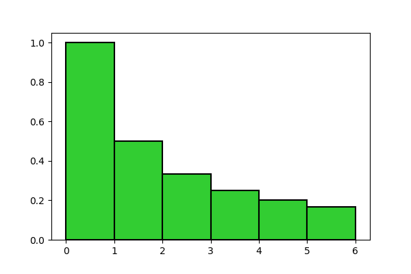
We can see each term as the area of a rectangle having the term itself as height and 1 as base. For example, for n = 6, sum (2) is just the area of the following bar chart:
In order to compute the area, that we’ll indicate with A, we can apply the Lemma of bar chart area, in its second form (Lemma N.5), which states that
Recall that, in the cited Lemma, the function C(n) computes the sum of the first n bar chart bases, while the function f(n) returns the heights of the individual rectangles; in addition \overline{C} and \widetilde{f} are respectively the simple extension of C and a C^1 extension of f. Let’s see what these functions are in our case.
Since all bases are unitary, the sum of the first k bases is simply k, hence
Its simple extension \overline{C} is the function shown in Figure 1 of the post From integer numbers to real numbers, that we show again here for convenience:
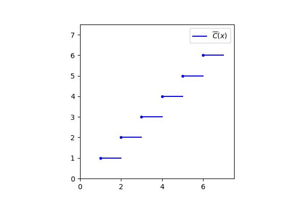
But we already know this function: it’s the integer part rounded down (or simply “integer part”):
If we wanted to prove it, we would have to formally define the integer part and compare it with the definition of simple extension, but it would be a mere formal exercise, which we can disregard. Instead, it’s important to note how formula (5) is evident from the picture: for example the \overline{C}(t) function always assumes value 1 for all real numbers between 1 included and 2 excluded, that are just those ones that, rounded down to the immediately previous integer, are equal to 1.
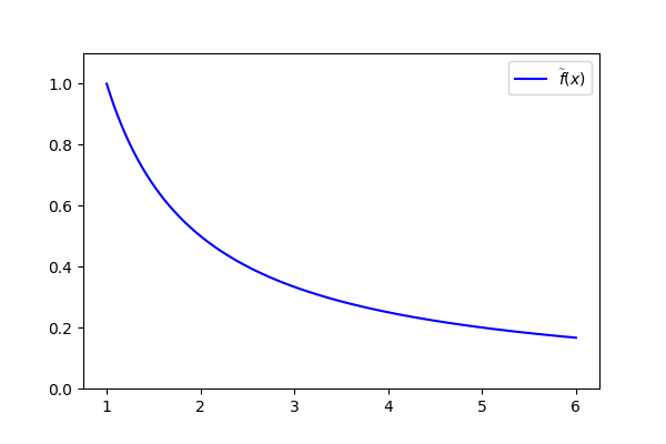
About function f, the one that computes the heights, in our case it’s
As an extension of it, we’ll take the most “natural” one:
that we can see in the following picture:
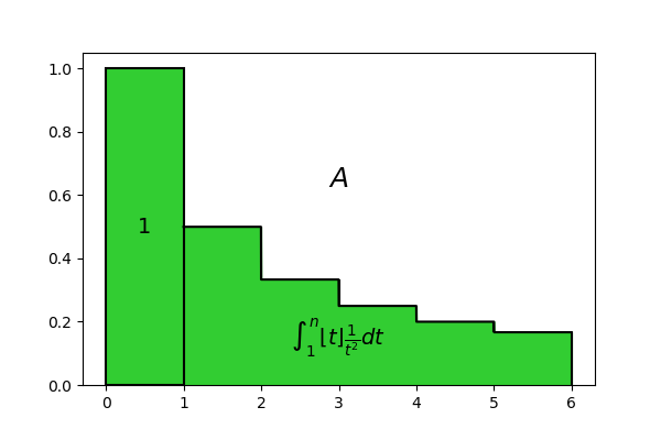
Placing formulas (4), (5), (6) and (7) into (3), we obtain:
Let’s try to understand better what this formula means. It computes the area of the bar chart shown in Figure 1, but looking at its expression carefully we can note that we decomposed this area into a sum, the first term of which is 1, and its second term is the integral \int_1^n \left \lfloor t \right \rfloor \frac{1}{t^2} dt. The 1 can be identified with the first rectangle, which has basis 1 and height 1, so the integral must be equal to the area of all the other rectangles altogether:
So we computed the area of the bar chart in Figure 1, but the formula we have found contains the integer part, which is not easy to operate with by analytical methods, because of its non-continuity. Let’s try to remove it. Doing so we obtain the following expression, the result of which we can call A^{\prime}:
This expression has a geometric interpretation similar to that of formula (8). Recall that the geometric meaning of the integral of a continuous positive function is the area of the figure obtained by projecting vertically the extremities of the function graph onto the horizontal axis. In this case, if we consider the graph of the function f(t) = \frac{1}{t} between 1 and n and project the points (1, f(1)) and (n, f(n)) onto the horizontal axis, we obtain a figure with an area equal to the integral \int_1^n \frac{1}{t} dt. Then if we take this figure and our rectangle with unitary area and put them near with each other, we obtain a figure very similar to the previous one, the area of which is just the number A^{\prime} = 1 + \int_1^n \frac{1}{t} dt:
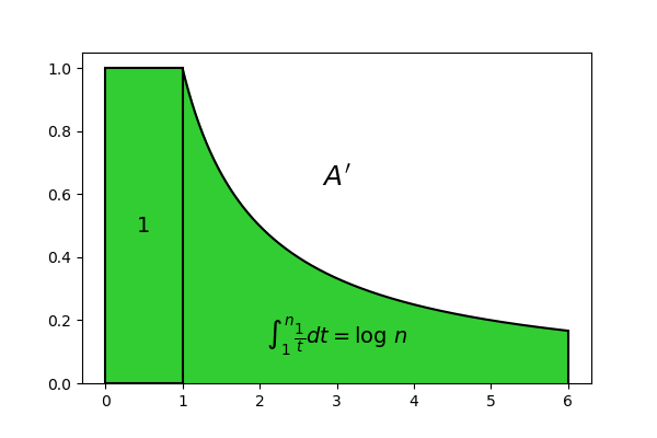
With respect to Figure 4, rectangles from the second on have been replaced by the graph of the function f(t) = \frac{1}{t}. The areas of the two figures seem to be quite similar, sufficiently for taking A^{\prime} as an approximation of A. The advantage is that A^{\prime} is far more simple to compute:
where the logarithm base is the Napier’s constant e (and in this case we are used not to indicate it explicitly, following a rather common convention).
Using A^{\prime} as an approximation of A, we can write:
If we overlap Figures 4 and 5, we can see the difference between the two areas, and so the error we make with this approximation:
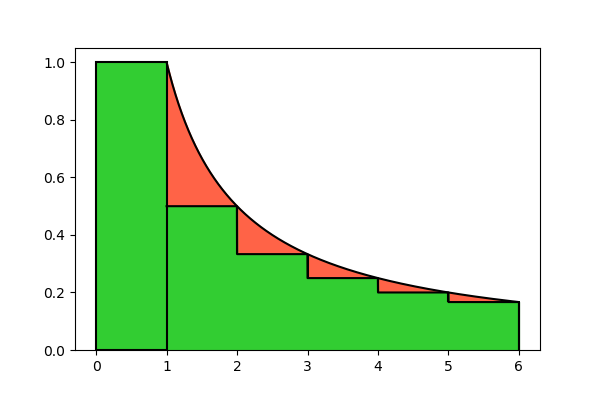
We can note that the graph of the function f(t) is always above the rectangles, so A^{\prime} \gt A. Hence (9) is an approximation by excess. In order to quantify how much it’s by excess, we should estimate the whole area of the red parts, that make up the difference between A and A^{\prime}. We’ll consider this area to be negative, because it must be subtracted from the estimate A^{\prime} in order to obtain the exact value A:
The estimation of the area of the red parts is simpler than it seems. In fact they get smaller so quickly, going towards right, that it’s not so wrong to sum them all up to infinity, and take this infinite sum as an approximation:
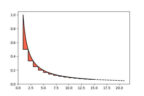
This figure, though extending to infinity towards right, has a finite area. The misure of this area can be obtained experimentally and, rounded up to the first two decimal digits, is 0.42. So we can refine our approximation as follows:
The new constant term 0.58 we obtained by subtracting 0.42 (the area of the infinite small red parts stripe) from 1 (the area of the first rectangle) is known as Euler’s constant and it’s denoted with \gamma. So we can ultimately write
We can translate this formula graphically as follows:
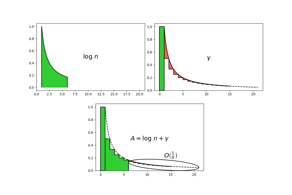
In Figure 8 it’s clear that it’s an approximation by default, since the error, highlighted in the picture, in a negative area (in red).
We have yet to understand how good this approximation is. Using the tools of asymptotic analysis, it can be proved that error is a big Oh of \frac{1}{n}, i.e., indicating it with h, |h| \leq \frac{K}{n}, for some constant K. The value of the expression \frac{K}{n} decreases as n increases, so the approximation improves for bigger numbers (you can realize that by looking at Figura 8: in fact, if n increases, the red parts stripe representing the error becomes thinner and thinner). Taking that into account, we can phrase the following asymptotic version of (11):
We can note that both (11) and (12) are approximated formulas; but while in (11) the error is generic, hidden in the approximated equality symbol (\approx) and completely unknown, in (12) it not only becomes explicit, but we at least know its asymptotic behaviour. Depending on cases, we’ll adopt both forms as our approximation of bar chart area:
Approximation of the sum of inverses of the first positive integers
For all integers n \gt 0:
where logarithm base is Napier’s number e, while \gamma \approx 0.58 is the Euler’s constant. In particular:
In addition to what expressed above, two things remain to be proved:
- That Figure 7, the infinite stripe of the red parts, has a finite area
- That the error of approximation (11) is asymptotically O(\frac{1}{n})
Let’s begin to express with a formula the area of Figure 7. To achieve this, let’s start from the area of the red parts of Figure 6. As you can easily see comparing Figures 4 and 5, this area is given by:
As n tends to infinity, we have that the area of Figure 7 is given by:
But every real number t differs from its integer part of less than a unity, that is t - \left \lfloor t \right \rfloor \lt 1. This lets to overestimate the integral as follows (considering that when the sign of \lt “goes outside” the integral, in general it becomes \leq):
This integral converges, because the associated series \sum_{n=1}^{\infty} \frac{1}{n^2} does too (we suppose you to be familiar with this principle, but in one of the next posts we’ll discuss about it from the number theory point of view). That means that Figure 7 has a finite area: we have completed the first point.
Concerning the error of approximation (11), comparing Figures 6, 7 and 8, you can see that it’s given by the area of that part of Figure 7 on the right of the last rectangle. With formulas:
The error made with the approximation (11) is thus exactly \int_n^{\infty} \frac{t - \left \lfloor t \right \rfloor}{t^2} dt, amount that we’ll indicate with h_n for highlighting the fact that it depends only on n. Let’s see how this error behaves asymptotically, as n increases. We can apply the same idea of passage (15): provided that, for all t, 0 \leq t - \left \lfloor t \right \rfloor \lt 1, we have that
The right side integral can be computed exactly:
So (16) can be rewritten as follows:
So it’s even more true that h_n = O\left(\frac{1}{n}\right), as we wanted to prove.
Alternatively, who is familiar with asymptotic relations may proceed more quickly as follows:
However the transfer of O(1) outside the integral is a property that should be proved and may lead to errors when not applied properly, so we recommend this technique only to the most expert people.
As we remarked in the post about Chebyshev’s Theorem, logarithms are of fundamental importance in number theory. Theorem N.6 is an additional confirmation of this, as it represents one of the fundamental blocks of the whole construction we’ll see in the next posts and that will bring us up to the prime number Theorem.
But Theorem N.6 has a great importance also for another reason: it’s where for the first time the natural logarithm appears, that is the logarithm having Napier’s number e for base. We’ll find it again almost always, from now on. Theorems where logarithm base is irrelevant, like Chebyshev’s Theorem, will be a few. In most Theorems the logarithm will have for base e, because one of the links of the argument chain that will bring us to them, will be just Theorem N.6.
Let’s try to use the approximation of Theorem N.6 for solving the “exercise” proposed initially, that is computing the number of terms of series (1) that are needed to be summed up in order to achieve at least 10. So let’s look for the smallest n such that:
We can use the approximation (13), thus modifying this unequality into:
Making some calculations, we obtain:
So, according to our estimation, in order to reach a sum of 10, n must be at least 12,406. Note that it’s an overestimation, being the correct number 12,368. You may object: “but didn’t we say that the estimation was by default?”. Indeed, the estimation of the bar chart area, that is the sum of the series, is by default, but just because the series sum is underestimated, more terms than necessary, according to the estimate, are required in order to achieve a fixed number, in this case 10. However, apart from the fact that the estimation of n is by excess, the obtained value is very close to the real one: we made an error of nearly 0.3%, and it can be further reduced by considering more decimal digits of the \gamma constant (we considered just two digits for simplicity).