Prerequirements:
The Prime Number Theorem is perhaps the most important theorem about prime numbers. It’s important first of all because it’s the result of a complex but fascinating operation: to make emerge order from chaos. It’s improper to say about chaos in mathematics, in which all is obtained by applying very precise rules, but it’s also true that when a numerical sequence escapes our immediate comprehension, many times it seems to have a chaotic nature. An example of such a sequence is the one of prime numbers. In fact, looking at a prime numbers table, it’s very simple to notice how their distribution seems to escape any regularity; instead it’s more difficult to note how behind this ostensible irregularity a precise order hides itself. In fact, if it’s true that irregularities are clear when you analyse the sequence of prime numbers in detail (for example looking at the difference between a prime number and the next one), things change when you observe it at a higher level, in its entirety. Making so you can note that the trend of the number of prime numbers less than or equal to an integer x, that is the value of the function we called \pi(x), it’s absolutely not chaotic, but as x increases it tends to adapt itself to a precise and very simple function: \frac{x}{\log x}. The Prime Number Theorem gives to this adaptation a precise mathematical meaning, the asymptotic equivalence:
Prime number Theorem
Applying Definition A.4 we can rephrase the statement of the Theorem as follows:
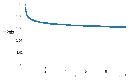
It’s not trivial to observe that this limit is 1, but it requires a great deal of abstraction, also because it’s not empirically evident, even for numbers of the order of hundred millions. In fact, as we saw about the strong version of Chebyshev’s Theorem, the ratio \pi(x) / \frac{x}{\log x}, for x = 100.000.000 still remains above 1.06:
Formula (1) clarifies the difference between the Prime Number Theorem and the strong version of Chebyshev’s Theorem. In fact, the only difference between the two theorems is that Chebyshev’s one does not establish the existence of the limit, but it restricts itself to say that if the limit exists, it must be 1. Instead the Prime Number Theorem adds the fact that the function \pi(x) / \frac{x}{\log x} tends to a limit, so stating its existence.
History and anecdotes
If it’s not simple to verify the Prime Number Theorem empirically, demonstrating it is even more difficult, indeed much more difficult. In fact the proof of this theorem is interesting in itself, also from a historical point of view, starting from the first research by Gauss in the late 18th century, continuing with Jacques Hadamard and Charles de la Vallée Poussin, who founded the first proof after one century, up to the so called “elementary” proof, that was found by Paul Erdős and Atle Selberg in 1949. For describing this historical excursus, we’ll use Paul Hoffman’s words. He, in The man who loved only numbers, tells it along with several anecdotes, clarifying at the same time the meaning of the term “elementary” (what follows is our translation from an Italian translation of the book):
The greatest victory on prime numbers was achieved by Erdős in 1949, but he didn’t like to talk about it, because it was a victory corrupted by debates. Though mathematicians don’t have any effective method for saying precisely where primes are, they know since late XVIII century a formula that describes their statistical distribution, showing how on average they thin out going on along numbers. Looking for such a formula, Carl Friedrich Gauss, probably the greatest mathematician of all time, began to study prime number tables in 1792, when he was fifteen. […] His hard work led Gauss in proposing the first formula that predicted the distribution of primes, but, though it was validated in the long list of known primes, the mathematician never proved that his Prime Number Theorem was universally true. A century passed before one proof of it was made by Jacques Hadamard and Charles de la Vallée Poussin. […] Proposed in 1896, it was based on a heavy equipment, and the best mathematical minds were certain that a proof could not be achieved by anything lighter. Erdős e Selberg, a colleague of his who didn’t achieved notoriety yet, astonished the world of mathematics with an “elementary” proof.
Elementary techniques do not necessarily mean simpler. In this context “elementary” means that the proof of the formula is based on a limited set of numbers, the so called real numbers, made up of integer numbers, rational numbers and irrational ones. […] The so called imaginary numbers, like \sqrt{-1}, also known as i, are not admitted.[…] Erdős didn’t have philosophical objections against imaginary numbers; simply, he preferred to limit his tools to the most familiar integer, rational and irrational numbers. He was the master of the elementary methods. When, in 1934, he went to visit Hardy, the latter believed that the Prime Number Theorem would never surrendered to elementary methods and, if it would, that all textbooks about number theory should be thrown away and be rewritten from the beginning. Hardy died in 1949, a few months before Erdős and Selberg used elementary methods to get rid of the Prime Number Theorem.
According to the friends of Erdős, the two colleagues planned to publish their essays side to side on a prominent magazine roughing out the respective contributions to the proof. Then Erdős began to send postcards to mathematicians informing them that he and Selberg had conquered the Prime Number Theorem. But Selberg, apparently, chanced upon a mathematician whom he didn’t know and who had received the postcard, and he was told “Did you know? Erdős and What’s-his-name have an elementary proof of the Prime Number Theorem”. He felt so offended, they tell, that he acted alone right away and published his essay without Erdős, so getting the majority of the credit for the proof. The Fields Medal, the equivalent of the Nobel prize for mathematics, was assigned to him only in 1950, and mostly for his work on the Prime Number Theorem.
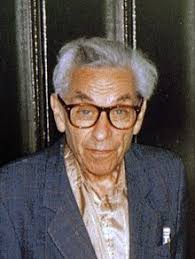
Eventually texts about number theory have not been rewritten from the beginning, as Hardy thought, perhaps because the proof of Erdős and Selberg is elementary from the point of view of the employed techniques, but it’s very complex in structure. Perhaps Hardy, when he made such a statement, imagined a proof at the same time elementary in techniques and also rather simple in structure, and he partially would have changed idea if he had seen the one of Erdős and Selberg. In spite of that, this proof created quite a stir when it was published and today it still remains of great interest for the employed techniques. Attempting to capture Hardy’s spirit, in the following posts we’ll try to rewrite it, in such a way that it will be clear what are the main passages and why at certain points is necessary to employ particular techniques. So perhaps Erdős, the “master of elementary methods”, will be able to teach us something about elementary methods that normally is not part of the programs of academic courses. We wanted to dedicate to him the main picture of this post, for contributing to release him from the stance of Selberg, who, as we saw, decided to publish the proof without his colleague.
If you want to read more about the history of the Prime Number Theorem, we recommend this interesting paper by D. Goldfeld: The elementary proof of the Prime Number Theorem: an historical perspective.
Strong version
Like for Chebyshev’s Theorem, also for the Prime Number Theorem there is a stronger form, where the function that approximates \pi(x) is called \mathrm{Li}(x):
Prime number Theorem, strong version
Where Li stands for Logarithmic integral and the function \mathrm{Li} is defined as follows:
Function \mathrm{Li}: logarithmic integral
We define the function \mathrm{Li}: \mathbb{N}^{\star} \rightarrow \mathbb{R}, called logarithmic integral, such that for all x \in \mathbb{N}^{\star}:
Theorem N.9 is a stronger version of Theorem N.8 for two reasons:
- As usual, the stronger version entails the weaker one: if the first is proved, the second turns out to be proved as well. In this case it can be proved that \mathrm{Li}(x) \sim \frac{x}{\log x}, so if the strong version of the Prime Number Theorem is true, i.e. if \pi(x) \sim \mathrm{Li}(x), then by transitivity \pi(x) \sim \frac{x}{\log x}, that is the weak version.
In order to understand why \mathrm{Li}(x) \sim \frac{x}{\log x}, we have to start from the following asymptotic expression of \mathrm{Li}(x):\mathrm{Li}(x) \sim \frac{x}{\log x} \sum_{k=0}^{\infty} \frac{k!}{(\log x)^k} = \frac{x}{\log x} + \frac{x}{(\log x)^2} + \frac{2x}{(\log x)^3} + \frac{6x}{(\log x)^4} + \ldots \tag{2}The proof of this formula requires quite some theory, that we set aside for the moment. Assuming the validity of (2), by Definition A.4 we’ll have that:
\lim_{x \to \infty} \left( \frac{x}{\log x} + \frac{x}{(\log x)^2} + \frac{2x}{(\log x)^3} + \frac{6x}{(\log x)^4} + \ldots \right) / \mathrm{Li}(x) = 1 \tag{3}In order to prove that \mathrm{Li}(x) \sim \frac{x}{\log x}, we have to prove that \lim_{x \to \infty} \frac{x}{\log x} / \mathrm{Li}(x) = 1. This comes from the fact that the terms after the first one that appear at the numerator of (3) have a lower order of magnitude than the first term, so they are irrelevant for the limit calculation.
Let’s see the passages in detail. We can rewrite (3) as follows (for the sake of brevity we’ll write simply \lim instead of \lim_{x \to \infty}):
\begin{aligned} \lim \left( \left( \frac{x}{\log x} + \frac{x}{(\log x)^2} + \frac{2x}{(\log x)^3} + \frac{6x}{(\log x)^4} + \ldots \right) / \frac{x}{\log x} \right) \cdot \left( \frac{x}{\log x} / \mathrm{Li}(x) \right) = 1 & \Leftrightarrow \\ \lim \left( \begin{gathered} \frac{x}{\log x} / \frac{x}{\log x} + \frac{x}{(\log x)^2} / \frac{x}{\log x} + \\ \frac{2x}{(\log x)^3} / \frac{x}{\log x} + \frac{6x}{(\log x)^4} / \frac{x}{\log x} + \\ \ldots \end{gathered} \right) \cdot \left( \frac{x}{\log x} / \mathrm{Li}(x) \right) = 1 & \Leftrightarrow \\ \lim \left( 1 + \frac{1}{\log x} + \frac{2}{(\log x)^2} + \frac{6}{(\log x)^3} + \ldots \right) \cdot \left( \frac{x}{\log x} / \mathrm{Li}(x) \right) = 1 \end{aligned} \tag{4}The limits of the terms \frac{1}{\log x}, \frac{2}{(\log x)^2}, \frac{6}{(\log x)^3}, … are all zero, thus the limit of the whole series inside parentheses exists and is 1. If we call this series S, by (4) we have that \lim S \cdot \frac{x}{\log x} / \mathrm{Li}(x) = 1. But we know that \lim S = 1, so from the limit of the product S \cdot \frac{x}{\log x} / \mathrm{Li}(x) we can obtain the limit of the other factor:
\lim \frac{x}{\log x} / \mathrm{Li}(x) = \lim \frac{S \cdot \frac{x}{\log x} / \mathrm{Li}(x)}{S} = \frac{\lim S \cdot \frac{x}{\log x} / \mathrm{Li}(x)}{\lim S} = \frac{1}{1} = 1So \lim \frac{x}{\log x} / \mathrm{Li}(x) = 1, that is \mathrm{Li}(x) \sim \frac{x}{\log x}.
- In addition, the second reason why Theorem N.5 is a stronger version of Theorem N.8 is that the ratio between \pi(x) and \mathrm{Li}(x) tends to 1 much more quickly than the ratio between \pi(x) and \frac{x}{\log x} (at Wikipedia there is a comparison table).
It may sound strange that two different functions, \mathrm{Li}(x) and \frac{x}{\log x}, are asymptotically equivalent to the same function \pi(x). The case of polynomials can help us to understand this situation better. By Definition A.2, two polynomials are asymptotically equivalent when they have the same degree and the same leading coefficient, i.e. the same term of highest degree. For example the polynomials 2x^3 and 2x^3 + x^2 - 3 are asymptotically equivalent, though they are different. We can say that the terms the degree of which is lower than the maximum one are irrelevant from the asymptotic equivalence point of view. The same thing happens for the functions \frac{x}{\log x} and \mathrm{Li}(x). The latter in fact, by (1), is given by the first plus a series of terms of lower “degree”, i.e. having a lower order of magnitude. Thus the two functions, just like the polynomials 2x^3 and 2x^3 + x^2 - 3, are asymptotically equivalent; so, as we said before, if one of them is proved to be asymptotically equivalent to \pi(x), by transitivity the same thing holds also for the other one.
According to some authors, the “Prime Number Theorem” is Theorem N.9, that is the strong version. This is indeed the first form of the theorem that was proved, by Hadamard and de la Vallée Poussin, as we saw in the previous section. The version proved by Erdős e Selberg in an “elementary” way is instead the weak one, so in the next posts we’ll focus on it.