Prerequirements:
- Row computation in second order linear dashed lines
- Row computation in third order linear dashed lines
- Dashed line theory definitions and symbols
This post can be considered as supplementary to those ones about row computation. In fact it’s worth, before passing to the formulas of \mathrm{t\_value}, pausing and looking closely to the moduli introduced with row computation, for example moduli (1) e (4) of the post Row computation in second order linear dashed lines. In fact they have a very precise meaning related to the dashed line: they are directly connected with the difference between the value of a dash and the one of the previous dash of another row. We’ll see all that in detail both for the second and the third order.
Difference between values of a dash of row i and the previous one of row j, in linear second order dashed lines
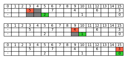
Let’s resume Figure 1 of the post Row computation in second order linear dashed lines:
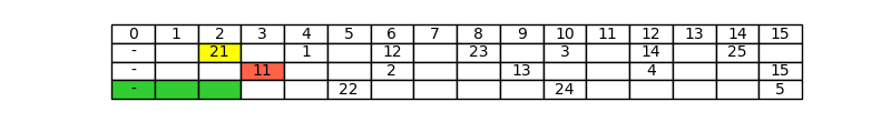
Let’s look, for each dash of row 1, at the value of modulus (1). Looking carefully, you can note a particular coincidence: the modulus value is just the number of columns that separate the considered dash of the first row, from the previous dash of the second row. For example the first dash, with value 3, has modulus 2 (in the sense that formula (1) gives 2 for x = 1) and in fact between it and the previous dash of the second row there are exactly two columns. This is true in all cases, even when the modulus value is 0 (i.e. there are no columns between the dash of row 1 and the previous dash of row 2), and when in the interposed columns there are other dashes of row 1:
We can note that, given any dash of the first row, the previous dash of the second row cannot be in the same column, but at most in the immediately preeceding column. In fact, if it was in the same column, it would be following in the ordering, since it has a greater row index. For example, the dash of the second row that precedes the one with corresponding modulus 4, as you can see in Figure 2, is the dash with modulus 6, not the one with modulus 7 that stays in the same column. This way the concept “number of columns separating a dash of the first row and the previous dash of the second row” is well defined, because it assumes the two dashes to be in different columns: at most they can stay in adjacent columns, and in that case the number of columns separating them is 0.
If the number of columns that separate a dash of the first row from the previous of the second row is given by modulus (1), by adding 1 we’ll obtain the difference between their values (with reference to Figure 2, these differences are, from top to bottom, 3, 1, 4, 2 and 5):
In this expression there is a -1 inside the modulus and a +1 outside: you could ask if they can be simplified, obtaining n_1 x \mathrm{\ mod\ } (n_1 + n_2). The answer is that this simplification is possible, but only in this particular case. In fact, given any two natural numbers a and b, it’s not always true that (a - 1) \mathrm{\ mod\ } b + 1 = a \mathrm{\ mod\ } b. The correct equality is the following (Teoria dei tratteggi (Dashed line theory, in Italian), Property 2.15, pages 61-62):
Using the special notation modulus star“, we can rewrite (2) in a more compact way:
However, as we have mentioned, it’s not a mistake to simplify (2) also as
but this second simplification is possible only because it can never happen that n_1 x \mathrm{\ mod\ } (n_1 + n_2) = 0 (see the following details for the proof), in which case, by definition of modulus star, (3) and (4) would assume different values. However, we’re going to prefer form (3) by affinity to what happens in the third order, as we’ll see in the next section.
Why can it never happen that n_1 x \mathrm{\ mod\ } (n_1 + n_2) = 0?
If n_1 x divided by n_1 + n_2 had remainder 0, the previous integer, n_1 x - 1, would have remainder n_1 + n_2 - 1. So modulus (1) would have value n_1 + n_2 - 1. But by formula (8) of Theorem T.2 (Computation of the x-th dash row in a second order linear dashed line), since by hypothesis the x-th dash is in row 1, this modulus must be less than n_2, so it can never be n_1 + n_2 - 1.
Summarizing, we can say that formula (3) computes the difference between the value of the x-th dash of the dashed line (n_1, n_2), if it belongs to the first row, and the previous of the second row.
But what if the x-th dash belongs to the second row?
As you can imagine, in this case the other modulus we introduced with row computation for second order linear dashed lines:
But this case is simpler, because modulus (5) immediately gives the difference between the values of the two dashes (not the number of columns between them), as you can see in the following picture:
Summarizing, we can state the following Theorem and the following Lemma:
Difference between the value of a dash of row i and the previous of row j, in a second order linear dashed line
Let T = (n_1, n_2) be a second order linear dashed line. Let x \gt 0, t := \mathrm{t}_T(x) and i be the row index of t. Let j be such that \{i, j\} = \{1, 2\}. Then the difference between the value of t and the one of the previous dash of row j is given by:
Equality between (n_1 x - 1) \mathrm{\ mod\ } (n_1 + n_2) + 1 and n_1 x \mathrm{\ mod^{\star}\ } (n_1 + n_2)
Let n_1, n_2 and x be integers, with n_1 \gt 1, n_2 \gt 1 and x \geq 0. Then the following equality is true:
We can note that Theorem T.3 lets us compute the difference between the values of two dashes, but these values are unknown. Only the ordinal and the row of the last of the two is known (by the way, the row can be computed from the ordinal thanks to Theorem T.2, so you could start also just from the ordinal). In one of the next posts we’ll see the theorems for computing the value of a dash, but Theorem T.3 shows us that it’s possible to say something not trivial about dash values without computing them.
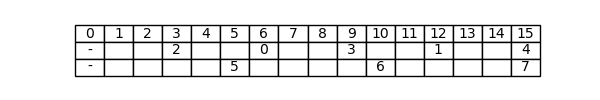
In the example of the post Row computation in second order linear dashed lines we saw that the eighth dash of the dashed line (3, 5) belongs to the second row. Applying Theorem T.3, we can compute the difference between the value of this dash and the one of the previous dash of the first row.
Applying the formula concerning the case t \in T[2] with (n_1, n_2, x) = (3, 5, 8), we have:
We’ve obtained 0: that means the two dashes have the same value, that is they are in the same column, as you can see in Figure 3 of the cited post, reported here for convenience:
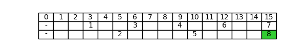
Note that in this example the employment of the \mathrm{\ mod\ } operator instead of \mathrm{\ mod^{\star}\ } is essential: if we used the second operator, the result would be, erroneously, 8.
A direct consequence of Theorem T.3 is the following Corollary:
Difference between the value of a dash of row i and the next of row j, in a second order linear dashed line
Let T = (n_1, n_2) be a second order linear dashed line. Let x \gt 0, and t := \mathrm{t}_T(x) belonging to row i. Let j be such that \{i, j\} = \{1, 2\}. Then the difference between the value of t and the one of the next dash of row j, is given by:
Let’s denote with t_p (where “p” stands for “previous”) the dash before t in row j, and with t_s (where “s” stands for “successive”) the one that follows it (still in row j):
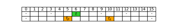
Moreover, let
- d_{tot}: distance between t_s and t_p;
- d_{prev}: distance between t and t_p;
- d_{succ}: distance between t_s and t;
By construction, we have:
By definition, d_{prev} is the distance between the dash t of row i and the one that preceeds it in row j, so, by Theorem T.3, we have that
hence
But d_{tot} is the distance between two dashes of row j, which is equal to n_j:
hence
that was the thesis to be proved.
Difference between the value of a dash of the first row and the ones of the previous dashes of the other rows
Similarly to what we’ve seen for the second order, the moduli that appear in formulas (5), (8) e (10) of the post Row computation in third order linear dashed lines, not only tell us which row the x-th dash belongs to, but tell us also something about its position with respect to the other dashes of other rows. This information is located into the numbers a and b by means of which the aforementioned moduli are expressed as elements of R_T(i). In fact the following Theorem is true:
Difference between the value of a dash of a row and the one of the previous dashed of other rows, for a third order linear dashed line
Let T = (n_1, n_2, n_3) be a third order linear dashed line. Let x \gt 0, t := \mathrm{t}_T(x) and i be the row index of t (obtainable by applying Theorem T.4 (Computation of the row of the x-th dash for a third order linear dashed line with two by two coprime components)). Let \{i, j, k\} = \{1, 2, 3\}. Let a and b be the integers, that exist by Theorem T.4, such that
Where N and R_T(i) are defined as in Theorem T.4. Then:
- a is the difference between the value of t and the one of the previous dash of row k
- b is the difference between the value of t and the one of the previous dash of row j
Theorems T.4 and T.5 are tightly connected. By Theorem T.4, if the x-th dash belongs to row i, then the modulus (n_j + n_k) n_i x \mathrm{\ mod\ } N belongs to the set R_T(i). But if it does, then by definition of R_T(i) it can be written in the form n_j a + n_k b, where a and b satisfy the constraints set by the definition itself (formulas (4), (7) and (9) of the post Row computation in third order linear dashed lines). Theorem T.5 goes one step forward: these a and b not only exist, but have a specific meaning. They are the differences between the value of the x-th dash and the ones of the previous dashes of the other rows. We can note that, if this is true, then a and b are also unique. In fact, both the previous dash of row k and the one of row j are univocally given: we don’t speak about “one” previous dash, but “the” previous dash, that is the greatest of the previous ones, that is just one. As a consequence, also the numbers a and b, that are the differences between the value of t and the one of these two dashes, are univocally given, that is the following stronger version of formula (5 + 8 + 10) of the cited post is true:
Getting back to the statement of Theorem T.5, we can also note that in (6) the coefficient of one component indicates the difference with the value of the previous dashes in the row of the other component: a, which is the coefficient of n_j, indicates the difference with the value of the previous dash of the row of n_k, and vice versa. This is important for not confusing a and b with each other, avoiding in the same time more complex notations (for example we could write n_j d_k + n_k d_j, where d_{\cdot} would indicate the difference with the value of the previous dash of the row in the subscript; but the simple mnemonic rule we pointed out makes such a notation unnecessary).
Lastly, we note that in this theorem, contrary to Theorem T.4, there isn’t the hypothesis that the components are two by two coprime: it is true for any third order linear dashed line.
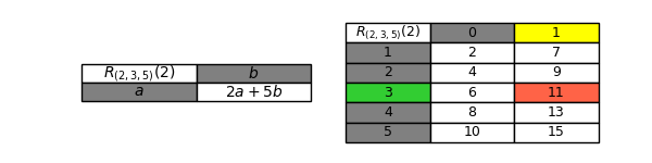
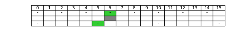
Let’s resume the example of the post Row computation in third order linear dashed lines and see what else we can say, thanks to Theorem T.5, about the sixth dash of T = (2, 3, 5), that we can call t. We saw that modulus (n_1 + n_3) n_2 x \mathrm{\ mod\ } N for this dashed line, for x = 6, is 2; in addition this number can be written in the form 2 = 2 a + 5 b,\ a \in \{1, 2, 3, 4, 5\},b \in \{0, 1\} as:
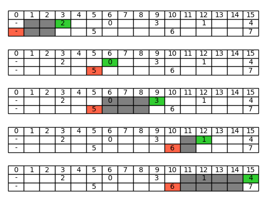
Using the mnemonic rule of the previous remark, we have that the coefficient of the component 2, that is 1, is the difference between the value of t and the one of the previous dash of the row of the component 5; conversely, the coefficient of the component 5, 0, is the difference between the value of t and the one of the previous dash of the row of component 2. In other terms, the first couple of dashes lays in adjacent columns, the second in a single column:
For checking other cases, we can explicitly construct the whole set R_T(2), representing all possible values of modulo (n_1 + n_3) n_2 x \mathrm{\ mod\ } N for the dashes in the second row. To do this, we can start from the definition (formula (7) of the post Row computation in third order linear dashed lines) and write into a table the values obtained as the parameters a and b vary:
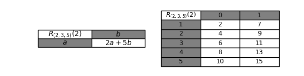
At this point, searching in the table the modulus of any dash of the second row, we are able to immediately “decompose” the modulus into the two parameters we called a and b, thus obtaining the value differences with respect to the previous dashes of the other rows: