13. Computation of spaces in second order linear dashed lines

Let T = (n_1, n_2) be a second order linear dashed line, x a fixed positive integer, and s := \mathrm{t\_space}_T(x). Then:

• Being s the x-th space of T, the first s columns of T can be divided into x spaces and s - x columns containing at least one dash
• Among the s - x columns containing at least one dash, only the ones divisible by both n_1 and n_2, that are the ones divisible by \mathrm{lcm}(n_1, n_2), contain two dashes; the other ones contain only one dash.

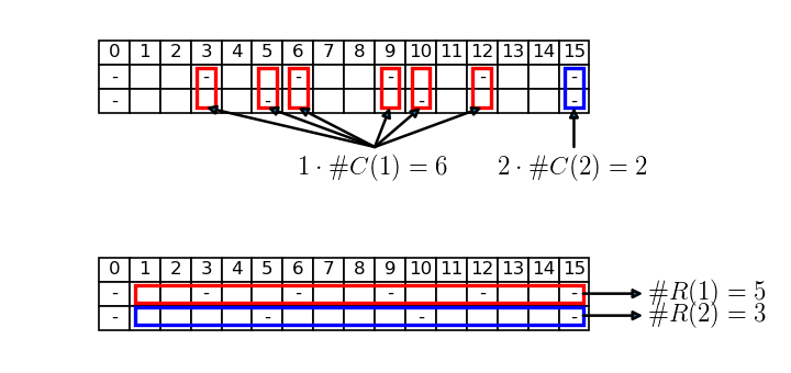
Let’s ask ourselves now: how many dashes are there in the first s columns of T? In order to answer this question, it’s possible to count dashes in at least two manners: by columns and by rows.

• If we count dashes by columns, we have to count 1 for every column containing only one dash, and 2 for those ones containing two dashes (more than two is not possible, because the dashed line has order two).
• If instead we count dashes by rows, we have to sum up the number of dashes in the first row, with the number of dashes in the second row, in both cases limiting ourselves to those ones with value less than or equal to s. We can compute these numbers by applying Proposition T.2 (Count of dashes up to a certain value in a first order linear dashed line).

So, making some calculations, we can obtain two different formulas that however, since they compute the same amount of dashes, can be equalized, originating the following equation:

As we noted about first order dashed lines, when counting dashes by rows we can stop at column s - 1 instead of s, because the latter is a space by hypothesis. In other terms, by applying Proposition T.2 and its Corollary, we’ll have that

Condition (7) can be in turn expressed by saying that s is a space of T:

Joining formula (6), where for improving readability we bring all the integer parts to the right, with the condition that s is a space of T, that we characterized in the previous Proposition, we’ll obtain the equation we call characteristic equation of second order linear \mathrm{t\_space}:

For simplicity we call “equation” formula (8) even if it’s, actually, an equation joined with a constraint about its solutions.

Before seeing the formula for computing \mathrm{t\_space}, let’s stop for a while, for answering the following question that we’ll often find later: “how many spaces are there in a period of a second order linear dashed line?”.
First of all this question makes sense because, by the Corollary of Property T.3 (Number of spaces in a period), all the periods of a periodical dashed line have the same number of spaces, and linear dashed lines are periodical, by Property T.4. We can say, in other terms, that the answer does not depend on the chosen period, but only on the dashed line. Since this number will often appear later, it’s convenient to give it a name:

If T is a second order linear dashed line, the number S(T) is given by the following Property:

If you try to compute the \mathrm{t\_space} function by solving the characteristic equation (8), you can soon realize that the term causing most problems in calculations is - \left \lfloor \frac{s}{\mathrm{lcm}(n_1, n_2)} \right \rfloor. However, this term is the smallest in absolute value among the terms with the integer part, being the one with the greatest denominator. So as a first step we may think about disregarding it, thus obtaining the equation:

The unknown is always s, that now is no more \mathrm{t\_space}_T(x), but something similar, as we specify with the following Theorem:

The proof is rather complicated and you can find it in Teoria dei tratteggi (Dashed line theory, in Italian), pages 208-220. However, the important thing, rather than the proof, that is very technical, is to understand the sense of the statement. First of all the function \mathrm{t\_space}_T^{\prime} is of some interest, because it’s a “space generator”. In fact Theorem T.12 states that the result of formula (11) is a space, being the solution of equation (8′) that, like (8), allows only spaces as solutions. Another interesting feature of the \mathrm{t\_space}_T^{\prime} function is that it generates spaces in an orderly fashion, being a function increasing in x.
Actually it’s not difficult to find functions with these features: some very simple examples are the functions \mathrm{lcm}(n_1, n_2) \cdot x - 1 and \mathrm{lcm}(n_1, n_2) \cdot x + 1, that return spaces for all x and are increasing in x. However these formulas generate a very scarce number of spaces, only one for each period of the dashed line, among S(T) total spaces. For example, considering the dashed line T = (3, 5), the only value assumed by the first function on the period from column 0 to column \mathrm{lcm}(n_1, n_2) - 1 = 14 is just \mathrm{lcm}(n_1, n_2) - 1 = 14, while in this period, like in any period, there are 8 spaces (we’ll check this with calculations in the next example). The virtue of the \mathrm{t\_space}_T^{\prime} function is to generate, instead, many spaces: it generates S(T) - 1 spaces for each period, skipping just one. We illustrate by an example this behaviour, that is a consequence of Theorem T.12 and we do not prove it for the moment.

Let’s consider the dashed line T = (n_1, n_2) = (3, 5). By Property T.7, the number of spaces in a period of the dashed line is S(T) = \frac{(n_1 - 1)(n_2 - 1) - 1}{\mathrm{GCD}(n_1, n_2)} + 1 = \frac{2 \cdot 4 - 1}{1} + 1 = 7 + 1 = 8. The function \mathrm{t\_space}_T^{\prime}(x) for this dashed line is the following:

\begin{aligned} \mathrm{t\_space}_{(n_1,n_2)}^{\prime}(x) & = \\ \mathrm{t\_space}_{(n_1)} \left( \left \lfloor \frac{(n_1 - 1)(n_2 x - 1) - 1}{(n_1 - 1)(n_2 - 1) - 1} \right \rfloor \right) & = \\ \mathrm{t\_space}_{(3)} \left( \left \lfloor \frac{2(5 x - 1) - 1}{2 \cdot 4 - 1} \right \rfloor \right) & = \\ \mathrm{t\_space}_{(3)} \left( \left \lfloor \frac{10 x - 3}{7} \right \rfloor \right) & = \text{[by Theorem T.1]}\\ \left \lfloor \frac{ 3 \cdot \left \lfloor \frac{10 x - 3}{7} \right \rfloor - 1 }{2} \right \rfloor \end{aligned}

The first 15 values assumed by this function, for x = 1, 2, 3, \ldots, are the following:

x	1	2	3	4	5	6	7	8	9	10	11	12	13	14	15
\mathrm{t\_space}_{(n_1,n_2)}^{\prime}(x)	1	2	4	7	8	11	13	16	17	19	22	23	26	28	31

Theorem T.12 states that, for each x, the number s := \mathrm{t\_space}_{(n_1,n_2)}^{\prime}(x) is a solution of equation (8′), which in our case is

\begin{cases} s - x = \left \lfloor \frac{s}{3} \right \rfloor + \left \lfloor \frac{s}{5} \right \rfloor \\ s \text{ is a space of }(3, 5) \end{cases} \tag{12}

For example, substituting the couple (x, s) = (8, 16) highlighted in bold in the table, we’ll have:

\begin{cases} 16 - 8 = \left \lfloor \frac{16}{3} \right \rfloor + \left \lfloor \frac{16}{5} \right \rfloor \\ 16 \text{ is a space of }(3, 5) \end{cases}

Indeed the equation is satisfied, since \left \lfloor \frac{16}{3} \right \rfloor + \left \lfloor \frac{16}{5} \right \rfloor = 5 + 3 = 8 = 16 - 8, and being 16 non divisible either by 3, either by 5. The same thing is true for the remaining couples of the table.

Representing these couples (x, s) together with the dashed line, we can see how in each period all the spaces, except the last one, are values assumed by the function \mathrm{t\_space}_{(n_1,n_2)}^{\prime}, i.e. are some “s“. In other terms, the function “skips” all the spaces of the kind \mathrm{lcm}(n_1, n_2) \cdot k - 1 = 15 k - 1:

The most interesting values of x are those that are part of the first case of Theorem T.12, i.e. those of the kind k (S(T) - 1) + 1, with k \gt 0: the first of such xs is S(T) and the next ones are 2 \cdot S(T) - 1, 3 \cdot S(T) - 2, etcetera. Let’s focus on the first one, obtained with k = 1, that in our case is 8. The cited Proposition states that, for x = 8, equation (8′) has two solutions, that are

k \cdot \mathrm{lcm}(n_1, n_2) \pm 1 = \mathrm{lcm}(n_1, n_2) \pm 1 = 15 \pm 1 = 14, 16 \tag{13}

We saw before the solution 16: it’s one of the values assumed by the \mathrm{t\_space}_{(n_1,n_2)}^{\prime} function, and we checked it to satisfy equation (8′), that in our case is (12). But the same equation is also satisfied by the other number:

\begin{cases} 14 - 8 = \left \lfloor \frac{14}{3} \right \rfloor + \left \lfloor \frac{14}{5} \right \rfloor \\ 14 \text{ is a space of }(3, 5) \end{cases}

We have that \left \lfloor \frac{14}{3} \right \rfloor + \left \lfloor \frac{14}{5} \right \rfloor = 4 + 2 = 6 = 14 - 8, and 14 is a space of the dashed line too, so also 14 is a solution of the equation. Theorem T.12 says that these cases, when the equation has a double solution, happens only when x is of the kind k (S(T) - 1) + 1, with k \gt 0; in addition, when this happens, the solution is given by formula (13), far simpler than the one that expresses \mathrm{t\_space}_{(n_1,n_2)}^{\prime}(x). However, even in these cases the formula for \mathrm{t\_space}_{(n_1,n_2)}^{\prime}(x) does not make a mistake, but it simply “choose” one of the two solutions, the biggest one. In fact, as we have seen, \mathrm{t\_space}_{(3,5)}^{\prime}(8) = 16 and not 14.

Now that we have seen in detail the \mathrm{t\_space}^{\prime} function, which in light of the previous example we can regard at all effects as an “approximated” \mathrm{t\_space} functions, thanks to a technical artifice we can construct the exact function. The mathematical details are in Teoria dei tratteggi (Dashed line theory, in Italian), pages 221-224, and the final result is the following:

In definition (14) there are two cases:

• The first case is when x is a multiple of S(T), that is x = S(T), 2 \cdot S(T), 3 \cdot S(T), \ldots. But, since every period of T has S(T) spaces, the S(T)-th space is the last space of the first period, the 2 \cdot S(T)-th space is the last of the second period, and so on. Then this case is helpful for computing the last space of each period. It’s not by chance that these spaces are exactly those “skipped” by the \mathrm{t\_space}^{\prime} function, as we saw in the previous example.
• In the second case we have that s_i(x) = s^{\prime}_i \left (x - \left \lfloor \frac{x}{S(T)} \right \rfloor \right ), i.e. the downcast function s_i employs its approximation, though introducing in its argument the term - \frac{x}{S(T)}, that is a “correction” for taking account of the skipped spaces.

In order to understand better definition (14), it’s worth first of all sketching it, identifying the three main functions involved:

• The function that maps x to \frac{x}{S(T)} (n_i - 1) \frac{\mathrm{lcm}(n_i, n_j)}{n_i}, that is involved in the first case; we’ll call it f_i
• The function that maps x to x - \left \lfloor \frac{x}{S(T)} \right \rfloor , that we’ll call g
• The function s^{\prime}_i

This way, formula (14) becomes:

s_i(x) := \begin{cases} f_i(x) & \text{if }S(T) \mid x \\ s^{\prime}_i(g(x)) & \text{otherwise} \end{cases} \tag{14'}

The role of the functions f_i, g and s^{\prime}_i, is clarified by the following example.

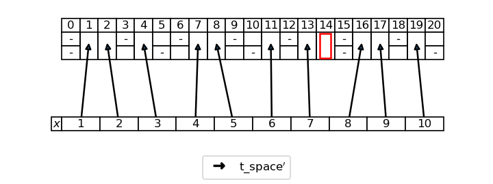
Let’s recall the dashed line T = (3, 5) of the previous example, having S(T) = 8. Applying definition (14′) with i = 1, we can compute the function s_1(x) for x = 1, \ldots, 11:

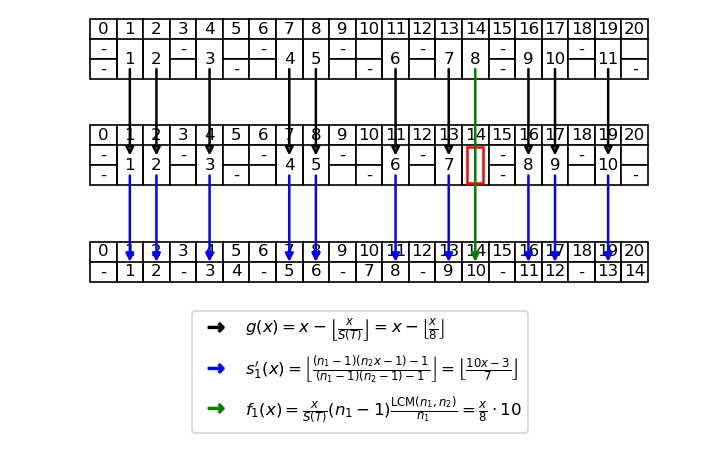
We can note that the aim of function g is to map the ordinal x referred to the dashed line T to the corresponding argument of function s^{\prime}_1, taking into account that the latter “skips” one space out of S(T), in this case one space out of 8. This way the downcast can be made for all spaces which are not the last of a period. For the other spaces, the corresponding first order ordinal is computed in a single step by means of the f_1 function (for example, in Figure 3 the ordinal 8 is mapped directly to ordinal 10). In fact, it could never be obtained by applying s^{\prime}_1, because it does not make part of its image (that are the numbers “reached” by the blue arrows).

Starting from Theorem T.13, we can obtain an explicit formula for computing the second order linear \mathrm{t\_space} function:

In the explicit form, the complexity of the formula for computing second order linear \mathrm{t\_space} is clearer. This complexity is also due to the presence of three nested integer part operations:

• the most external integer part comes from the first order function \mathrm{t\_space}_{(n_i)}
• the central one comes from the approximated downcast function s^{\prime}_i
• the most internal integer part is necessary in order to transform the approximated downcast function in the exact one