The proof strategy which will be exposed here has the goal of proving Hypothesis H.1 (Hypothesis of existence of Goldbach pairs based on dashed lines) through the properties of spaces. We have identified two different methods to do that:
- A method that uses a formula to explicitly calculate spaces;
- A method that uses the concept of maximum distance between consecutive spaces.
Both have as their starting point a reformulation of Hypothesis H.1, which is different in each case.
Method based on the explicit calculation of spaces
Suppose we are able to calculate exactly which are the spaces of a dashed line, with an algebraic expression depending on a variable x. The ideal thing would be to do it respecting the order, that is to calculate a function which, given x, returns the x-th space. Using such a function, which we will call \mathrm{t\_space}, it is possible to rewrite the two unknown spaces p and q of the Hypothesis H.1 respectively as \mathrm{t\_space}(x) and \mathrm{t\_space}(y). We thus obtain the following Hypothesis, in which the unknowns are no longer p and q, but x and y:
Hypothesis of existence of Goldbach pairs based on the function \mathrm{t\_space}
Let 2n \gt 4 be an even number and k be its validity order. Then there exist two positive integers x and y such that, with reference to the dashed line T_k:
- \mathrm{t\_space}(x) and \mathrm{t\_space}(y) are both within the validity interval;
- \mathrm{t\_space}(x) + \mathrm{t\_space}(y) = 2n.
This method, therefore, consists in proving that the equation \mathrm{t\_space}(x) + \mathrm{t\_space}(y) = 2n has at least one solution (x, y), for each 2n \gt 4. We will call this equation Goldbach’s equation on spaces:
Goldbach’s equation on spaces
Let 2n \gt 4 be an even number, and k the relative validity order. Then the following equation in the unknowns x and y, which refers to the dashed line T_k:
is called Goldbach’s equation on spaces.
The following image graphically represents this method, based on an example:
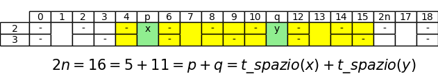
As you can guess, the difficulty of this method lies in expressing the function \mathrm{t\_space} through an algebraic expression, with the intention that, by replacing this expression in Goldbach’s equation on spaces, the latter becomes an algebraic equation in the variables x and y. This would lead the search for solutions to an algebraic calculation problem which, in principle, should be tackled with various tools, even elementary ones.
So, in order to achieve the goal, the steps would essentially be the following:
- Find a formula to calculate the function \mathrm{t\_space} for linear dashed lines of any order (although it would suffice to treat the case of dashed lines T_k, for any k);
- Rewrite Goldbach’s equation on spaces, using the formula just found;
- Prove that the equation thus rewritten has solutions;
- Prove that, for at least one of the solutions (x, y) identified, the relative values of \mathrm{t\_space}(x) and \mathrm{t\_space}(y) are in validity interval.
Finally you could apply Property T.1 (Spaces and prime numbers), which assures us that all spaces in the validity interval are also prime numbers, and thus the found solutions are also Goldbach pairs, which would complete the proof of the conjecture.
![]() Calculation of \mathrm{t\_space} for dashed lines of arbitrary order
Calculation of \mathrm{t\_space} for dashed lines of arbitrary order
Method based on the study of double dashed lines
It would be much easier to solve Hypothesis H.1 if, instead of finding the two spaces p and q, it would suffice to find only one of the two, say p. This would be possible if there were a mechanism to ensure that the integer q = 2n - p is itself a space, without setting this condition explicitly. This mechanism exists, but it relies on the use of a slightly more complicated dashed lines than the T_k dashed lines of Hypothesis H.1. Let’s see how it works.
The basic principle consists in limiting the possible choices of p, identifying conditions that guarantee that q is also a space. To find these conditions, we can start from the definition of space. If q must be a space, then it must not be divisible by any component of the dashed line, which in Hypothesis H.1 is T_k. Therefore q must not be divisible by p_1, \ldots, p_k, i.e. q \mathrm{\ mod\ } p_i must be different from 0, for each i=1, \ldots, k. The interesting aspect is that this condition on q, thanks to the Goldbach equation which links p and q, can be transformed into a similar condition on p. This follows from a general property of integers, expressed by the following Lemma:
Relationship between the moduli of two positive integers and the one of their sum
Let a, b and m be three positive integers. Then
We’ll denote with a^{\prime}, b^{\prime} and h^{\prime}, respectively, the quotients of the division of a, b and h by m, so a = ma^{\prime} + a \mathrm{\ mod\ } m, b = mb^{\prime} + b \mathrm{\ mod\ } m and h = mh^{\ prime} + h \mathrm{\ mod\ } m. Substituting into (1), we’ll have that:
By separating the modules from the other terms and highlighting m, we’ll get:
If a \mathrm{\ mod\ } m = 0, we’ll get:
In particular h \mathrm{\ mod\ } m - b \mathrm{\ mod\ } m is a multiple of m. But h \mathrm{\ mod\ } m and b \mathrm{\ mod\ } m, by definition of modulus, are both less than m, so their difference can vary from a minimum of -(m - 1) (when h \mathrm{\ mod\ } m = 0 and b \mathrm{\ mod\ } m = m - 1) to a maximum of m - 1 (when h \mathrm{\ mod\ } m = m - 1 and b \mathrm{\ mod\ } m = 0). Then the only multiple of m to which the difference h \mathrm{\ mod\ } m - b \mathrm{\ mod\ } m can be equal is 0, then b \mathrm{\ mod\ } m = h \mathrm{\ mod\ } m. But h = a + b, so b \mathrm{\ mod\ } m = (a + b) \mathrm{\ mod\ } m. Thus we have proved the rightward implication.
As for the other implication, assuming that b \mathrm{\ mod\ } m = (a + b) \mathrm{\ mod\ } m = h \mathrm{\ mod\ } m , substituting in (2) we’ll get:
In particular a \mathrm{\ mod\ } m is a multiple of m; but being, by definition of modulus, between 0 and m - 1, it can only be equal to zero. Thus the implication to the left is also proved.
Applying Lemma L.1 in our case, with a := q, b := p and m := p_i, and remembering that p + q = 2n, we’ll get:
From which, by negation, we get:
This is true for each p_i component, because no particular assumptions have been made about which component to choose. This means that the condition that q is a space, i.e.:
is equivalent to the following one:
The condition that q is a space was then translated into an equivalent condition on p. This way we can focus only on the single variable p.
Going back to Hypothesis H.1, we must also consider that p must be a space; so, in summary, p must satisfy two conditions:
- It must be a space;
- It must be such that q = 2n - p is also a space.
The first condition can be written as it has already been done for q:
The second condition, as we have seen, is given by (3). Putting together formulas (3) and (4), we’ll obtain the following formula:
It can be observed that p_1 = 2, so, in the first line, we have 2n \mathrm{\ mod\ } p_1 = 2n \mathrm{\ mod\ } 2 = 0; therefore the set \{0, 2n \mathrm{\ mod\ } p_1\} actually consists of only the number 0. This condition can be made explicit by separating the first row from the subsequent ones, obtaining:
For the lines related to p_2, \ldots, p_k the same situation as the first could occur: for a generic component p_i, for i = 2, \ldots , k, if p_i was one of the prime factors of n, 2n \mathrm{\ mod\ } p_i would be 0 and so the set \{0, 2n \mathrm{\ mod\ } p_i\} would reduce to the only element 0.
Based on the above passages, the following Proposition can be proved:
Characterization of Goldbach pairs formed by spaces of T_k
Let 2n \gt 4 be an even number and k the relative validity order. Then, given two positive integers p and q, the following conditions are equivalent:
- (p, q) is a Goldbach pair for 2n formed by spaces of T_k
- 1 \lt p \lt 2n - 1;
\begin{cases} p \mathrm{\ mod\ } p_1 \neq 0 \\ p \mathrm{\ mod\ } p_2 \notin \{0, 2n \mathrm{\ mod\ } p_2\} \\ \ldots \\ p \mathrm{\ mod\ } p_k \notin \{0, 2n \mathrm{\ mod\ } p_k\} \end{cases}
q = 2n - p.
- 1 \lt p \lt 2n - 1
- \begin{cases} p \mathrm{\ mod\ } p_1 \neq 0 \\ p \mathrm{\ mod\ } p_2 \notin \{0, 2n \mathrm{\ mod\ } p_2\} \\ \ldots \\ p \mathrm{\ mod\ } p_k \notin \{0, 2n \mathrm{\ mod\ } p_k\} \end{cases}
- q = 2n - p
First of all p cannot be 1, otherwise it wouldn’t be prime, so it couldn’t form a Goldbach pair. Being by hypothesis a positive integer, it must therefore be p \gt 1. The same reasoning can be repeated for q, so also q \gt 1. But, by Goldbach’s equation, p + q = 2n, so p = 2n - q, and being q \gt 1 we have p \lt 2n - 1. Thus we have proved (a).
We have seen that (b) is equivalent to assuming that p and q = 2n - p are both spaces of T_k, and this is true in point 1. of the statement, therefore also (b) is proved. Finally (c) is a different writing of Goldbach’s equation.
We now prove the converse, 2. \Rightarrow 1., that is, if (a), (b) and (c) hold, then (p, q) is a Goldbach pair for 2n formed by spaces of T_k, i.e.:
- p and q are spaces of T_k;
- p and q are prime;
- p + q = 2n.
(i) follows directly from (b), as seen earlier. Regarding (ii), for the Property T.1 (Spaces and prime numbers) it suffices to prove that p and q are within the validity interval, i.e. that p_k + 1 \leq p \leq p_k^2 - 1. This is true because:
- The smallest space of T_k greater than 1 is p_k + 1. In fact, if m is an integer between 2 and p_k, all its prime factors, being less than or equal to m, are less than or equal to p_k, so they coincide with one of the primes p_1, \ldots, p_k, which are the components of T_k. So m, being divisible by one of the dashed line components, is not a space. Assuming that 2 \leq m \leq p_k, none of these m can be a space, so the smallest space greater than 1 is greater than or equal to p_k + 1.
- Since k is the validity order relative to 2n, by definition we have that 2n \leq p_k^2 - 1; therefore, since (a) p \lt 2n - 1 \leq 2n, also p \leq p_k^2 - 1.
Finally, (iii) follows directly from (c).
To better understand formula (5), it is convenient to decompose the conditions of the type p \mathrm{\ mod\ } p_i \notin \{0, 2n \mathrm{\ mod\ } p_i\} into the two conditions p \mathrm{\ mod\ } p_i \neq 0 and p \mathrm{\ mod\ } p_i \neq 2n \mathrm{\ mod\ } p_i and order the conditions thus obtained as follows:
- p \mathrm{\ mod\ } p_1 \neq 0
- p \mathrm{\ mod\ } p_2 \neq 0
- \ldots
- p \mathrm{\ mod\ } p_k \neq 0
- p \mathrm{\ mod\ } p_2 \neq 2n \mathrm{\ mod\ } p_2
- \ldots
- p \mathrm{\ mod\ } p_k \neq 2n \mathrm{\ mod\ } p_k
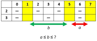
The first k conditions say that p must not be divisible by p_1, \ldots, p_k, i.e. that it must be a space of T_k. As an example let’s consider, for k = 4, the following dashed line:
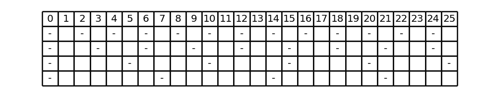
With reference to the representation of this dashed line, the values of p that satisfy the first k conditions correspond to the columns that do not contain any dash. In fact, on each line a dash is shown in correspondence with the values of p such that p \mathrm{\ mod\ } p_i = 0, i.e. that do not satisfy the i-th condition. So, conversely, if the ith condition is satisfied, then the column p doesn’t contain a dash on the row i and, extending to all lines, if all the first k conditions are satisfied, then column p does not contain any dash, on any line, i.e., by definition it is a space.
The same reasoning can be extended to the remaining conditions, obviously limiting ourselves to the cases where 2n \mathrm{\ mod\ } p_i \neq 0, because otherwise the condition p \mathrm{\ mod\ } p_i \neq 2n \mathrm{\ mod\ } p_i would be equivalent to the condition p \mathrm{\ mod\ } p_i \neq 0 already taken into consideration among the first k.
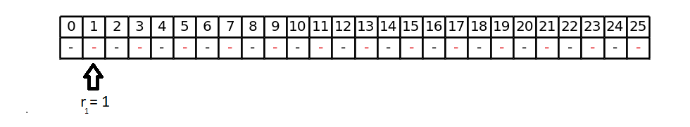
Let i \in \{2, \ldots, k\} such that 2n \mathrm{\ mod\ } p_i \neq 0. Consider the condition p \mathrm{\ mod\ } p_i \neq 2n \mathrm{\ mod\ } p_i. As we did for the first k conditions, we can fill our table by inserting a dash in correspondence with the columns of the i-th row so that this condition is not satisfied, i.e. the columns p such that p \mathrm{\ mod\ } p_i = 2n \mathrm{\ mod\ } p_i. In the expression 2n \mathrm{\ mod\ } p_i, n is constant, because it is half of the even number of which to look for Goldbach pairs, while p_i is not constant in general, but it is on the line i. Then the whole expression 2n \mathrm{\ mod\ } p_i is a constant of the line i, and for simplicity we will call it r_i. The condition p \mathrm{\ mod\ } p_i = 2n \mathrm{\ mod\ } p_i says that p must have this remainder r_i modulus p_i, with r_i \neq 0 by assumption. So on the line i we will have two sequences of dashes: the one of the columns with remainder 0 modulus p_i and the one of the columns with remainder r_i modulus p_i. The dashes of each sequence are equidistant from each other, but their co-presence on the same line results in a less regular drawing.
As we saw in Hypothesis H.1, we have to choose k as the smallest integer such that (p_{k+1})^2 \gt 100. Obviously the function (p_{k+1})^2 is increasing with respect to k, so we’ll just try increasing values of k until the value of the function exceeds 100. For k = 3 we have that (p_{k+1})^2 = (p_4)^2 = 7^2 = 49 \lt 100, while for k = 4 we have (p_{k+1})^2 = (p_5)^2 = 11^2 = 121 \gt 100, so the required value of k is k = 4.
Now let’s compute the r_i row constants:
- r_2 = 100 \mathrm{\ mod\ } p_2 = 100 \mathrm{\ mod\ } 3 = 1
- r_3 = 100 \mathrm{\ mod\ } p_3 = 100 \mathrm{\ mod\ } 5 = 0
- r_4 = 100 \mathrm{\ mod\ } p_4 = 100 \mathrm{\ mod\ } 7 = 2
Substituting into the list of conditions preceding Figure 2, we’ll get:
- p \mathrm{\ mod\ } p_1 \neq 0
- p \mathrm{\ mod\ } p_2 \neq 0
- p \mathrm{\ mod\ } p_3 \neq 0
- p \mathrm{\ mod\ } p_4 \neq 0
- p \mathrm{\ mod\ } p_2 \neq 1
- p \mathrm{\ mod\ } p_4 \neq 2
The condition p \mathrm{\ mod\ } p_3 \neq 0 was written only once but formally it would be duplicated, because replacing n in the condition p \mathrm {\ mod\ } p_3 \neq 2n \mathrm{\ mod\ } p_3, being 2n \mathrm{\ mod\ } p_3 = r_3 = 0, we’ll obtain again the third condition.
Overall, by inserting the dashes where indicated by the negation of the first four conditions, the previous Figure 2 is obtained, while also considering the other two final conditions, the following Figure is obtained (for the sake of brevity, we’ll continue to display only the portion of the table up to column 25, while for completeness we should arrive at 100):
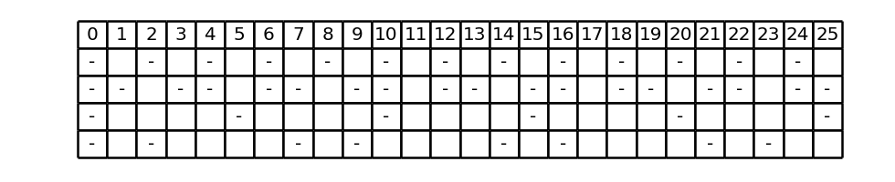
The columns of this new Figure that are without dashes represent the values of p which satisfy all the conditions of the previous list. But these values of p, if included between 1 and 2n - 1 excluded, by Proposition L.1 are precisely the values that are part of a Goldbach couple. For example, such a p is the number 11, because in Figure 3 column 11 contains no dashes. In fact, 11 just forms a Goldbach pair for 100, because 100 = 11 + 89 and 89 is also prime. The same is true for 17 and subsequent dash-free columns that would be displayed if we extended the table to 100: by construction, they all generate Goldbach pairs (100 = 17 + 83, etc.).
Figure 3 also represents a dashed line, even if structurally it is presented in a very different way from Figure 2, because dashes are not all equidistant from each other on all rows. The definition of dashed line is general enough to cover both cases; however, there are several specific types of dashed lines. The dashed lines represented by tables like the one in Figure 2, where the dashes are always at regular intervals and start from 0, are called linear dashed lines; instead those represented by a table like the one in Figure 3, where at least one row contains two sequences of equidistant dashes, one starting from 0 and the other starting from a constant r_i \neq 0, are called double dashed lines (by contrast, linear dashed lines are sometimes also called “single” dashed lines). The notions about double dashed lines that you need to know to understand this proof strategy will be introduced in this page shortly; however, a dedicated in-depth page is available:
The linear dashed line represented by Figure 2 is indicated, as we have seen, with the symbol T_4, because its components are the first 4 prime numbers (an alternative, more explicit notation is the one with the list of components, i.e. (2, 3, 5, 7)). The double dashed line represented by Figure 3 is instead indicated with the symbol T_4^{(0,1,0,2)}, where the quadruple (0,1,0,2) indicates, for each row, whether there is an additional sequence of dashes (when the element of the quadruple is different from 0) and, if so, where this sequence starts from. For example, in this case the second element of the quadruple is 1 because on the second row there is, compared to Figure 2, the sequence of additional dashes 1, 4, 7, 10, etc., where the dashes are always at intervals of p_2 = 3 columns, but starting from 1 instead of 0.
In general, if T is a dashed line with k rows and (r_1, r_2, \ldots, r_k) is a k-uple of non-negative integers and smaller than the corresponding components of the dashed line, the double dashed line obtained starting from T and adding, on the rows i for which r_i \neq 0, a further sequence of dashes starting from r_i, will be indicated with the symbol T^{(r_1, r_2, \ldots, r_k)}.
In the case of the proof strategy we are describing, as we have seen, the values of r_i are given by 2n \mathrm{\ mod\ } p_i (including r_1 which according to this formula is always 0: often, to make this thing explicit, we’ll write 0 directly instead of r_1). So we can reformulate Hypothesis H.1 as follows:
Hypothesis of existence of Goldbach pairs based on dashed lines (second form)
Let 2n \gt 4 be an even number and let k be its validity order. Let r_i := 2n \mathrm{\ mod\ } p_i, for each i = 2, \ldots, k. Then the double dashed line T_k^{(0, r_2, \ldots, r_k)} contains at least one space p such that 1 \lt p \lt 2n.
The definition of double dashed lines (which you don’t need to know in detail in this context) includes the constants r_i, but is not constrained by a particular value of them. The reason is that we want to approach the problem from a more general point of view: if we can prove the existence of spaces included in a certain interval (in our case (1, 2n)) in a double dashed line T^{(r_1, r_2, \ldots, r_k)}, where T is any starting linear dashed line and r_1, r_2, \ldots, r_k can be any, even more so we will have proved the existence of such spaces when T = T_k and r_i = 2n \mathrm{\ mod\ } p_i , which is what Hypothesis H.1 (second form) requires.
We certainly cannot expect all possible choices of r_i to generate double dashed lines that contain spaces in a certain interval. For example, if in a double dashed line a component is 2, i.e. all the even numbers on the corresponding row are dashes, we can just set the corresponding r_i = 1 to “close” all the remaining spaces, because this choice implies that all odd numbers are also dashes, so there would be no more spaces either on that row, or a fortiori in the whole dash (whatever the other components and their respective r_i are):
The double dashed line of Hypothesis H.1 (second form) has as its first component p_1 = 2, but fortunately r_1 = 0, so this problem does not arise; however our intent is to find conditions for which a generic double dashed line T^{(r_1, r_2, \ldots, r_k)} has spaces in a given interval. There are at least two methods for doing this: they are, if you like, sub-methods of the one based on the study of double dashed lines.
Method based on the approximate calculation of spaces
The first method is based on the following observation. After all, we already know what the interval in which we want to search for spaces looks like, that is (1, 2n); in particular, we know that the minimum is always 1, and that this minimum is excluded. Therefore, given a generic double dashed line D, the following possibilities can arise:
- 1 is a space. If so, it’s the first space, since 0 definitely isn’t. Returning to the initial notations, we therefore have that \mathrm{t\_space}_D(1) = 1. Then, if there are spaces between 1 and 2n excluded, among them there will certainly be the second one. So in this case we have to prove that \mathrm{t\_space}_D(2) \lt 2n.
- 1 is not a space. In this case, if there are spaces between 1 and 2n excluded, among them there will certainly be the first one, so in this case we have to prove that \mathrm{t\_space}_D(1) \lt 2n. However, let’s re-examine the condition of the previous case: if the second space were smaller than 2n, even more so the first space would be smaller. So, to prove that \mathrm{t\_space}_D(1) \lt 2n, we can prove that \mathrm{t\_space}_D(2) \lt 2n: in this case it is not a necessary condition, but it is sufficient.
As we have seen, in any case the condition \mathrm{t\_space}_D(2) \lt 2n would guarantee the existence of at least one space in the interval (1, 2n). This, if D is the double dashed line of Hypothesis H.1 (second form), would guarantee the truth of the Hypothesis itself, which can therefore be further reformulated:
Hypothesis of existence of Goldbach pairs based on dashed lines (third form)
Let 2n \gt 4 be an even number and let k be its validity order. Let r_i := 2n \mathrm{\ mod\ } p_i, for each i = 2, \ldots, k. Then the second space of the double dashed line T_k^{(0, r_2, \ldots, r_k)} is less than 2n.
This reformulation takes us back to the initial problem of calculating spaces, but this time in a double dashed line instead of a “single” dashed line. But, as we said, the explicit calculation of the spaces is very difficult already in single dashed lines, let alone double ones! However, in our case we don’t have to compute the second space exactly, we just have to prove that it is less than some fixed number; so even an approximate value would be fine, as long as we can guarantee that the real value does not deviate so much that it exceeds 2n. Generalizing, given a double dashed line D we can make a reasoning of this type:
- Suppose we find a function B(x) such that, for each x, \mathrm{t\_space}_D(x) \lt B(x)
- So, given a constant C, to prove that \mathrm{t\_space}_D(x) \lt C it suffices to prove that B(x) \lt C
The advantage, reasoning this way, would be that we can try to find a function B(x) that is much simpler to express algebraically, than the function \mathrm{t\_space}, making the second point simple. However, the complicated problem would be to find this function, as required by the first point. We thought of dealing with this problem in increasing degrees of difficulty, starting from single dashed lines for increasing orders, to then extend the results to double dashed lines. We have currently found the function B(x) for (single) linear dashed lines up to fourth order (the results will be soon available here).
Method based on the concept of maximum distance between consecutive spaces
While we previously focused on the minimum of the interval (1, 2n), let us now focus on its width. Seeing it as a real interval, we can say that its width is smaller than 2n - 1; it is smaller by an infinitesimal amount, being the interval interval open, however the width is strictly smaller than 2n - 1. Let us now consider the spaces of the double dashed line of the cited Hypothesis; in particular let’s consider the pairs of consecutive spaces: the first with the second, the second with the third, and so on. We calculate the differences (or distances, a term we prefer because it suggests a graphic representation) between these spaces. We will therefore have infinite distances: the second space minus the first, the third minus the second, and so on: it is an infinite sequence of integers. This sequence is limited, because there cannot exist two consecutive spaces arbitrarily distant (this derives from the fact that double dashed lines, like single ones, are periodic; thus, if s is a space, so is s + L, where L is the length of the period, so the space following s cannot be more than L columns far from it). But a limited sequence of integers admits a maximum, for which the following Definition is allowed:
Maximum distance between consecutive spaces of a dashed line
Let T be a dashed line. The maximum distance between two consecutive spaces of T will be indicated with the symbol \mathrm{MDS}(T).
Now, returning to Hypothesis H.1 (second form), suppose that \mathrm{MDS}\left(T_k^ {(0, r_2, \ldots, r_k)}\right) is less than 2n - 1. Then, if 1 is a space, certainly the interval (1, 2n) would contain another space of the dashed line, at least the second one. Indeed, if the second space were out of interval, it would be greater than or equal to 2n, so its distance from the previous space, which is 1, would be at least 2n - 1, in contrast to the assumption that \mathrm{MDS}\left(T_k^{(0, r_2, \ldots, r_k)}\right) \lt 2n - 1. This would allow to prove Hypothesis H.1 (second form) for all numbers 2n such that 1 is a space of the dashed line T_k^{(0, r_2, \ldots, r_k) }, that is, it is an element of a Goldbach pair for that number; thus Hypothesis H.1 would be proved for all numbers 2n of the form 1 + p, with p prime.
What if 1 isn’t a space? In this case it is necessary to prove that the first space is less than 2n. This can be done in at least two ways:
- Either with the previous method, setting x = 1 instead of 2.
- Or, in proving that \mathrm{MDS}\left(T_k^{(0, r_2, \ldots, r_k)}\right) \lt 2n - 1, also include a theoretical “space number 0”. This might look like a trick, but if we consider the known expressions of \mathrm{t\_space}(x) for first or second order linear dashed lines and we try to evaluate them for x = 0, it turns out that, whatever the starting dashed line is, \mathrm{t\_space}(0) = -1, however counterintuitive it may be. The known formulas for calculating the function \mathrm{t\_space} for linear dashed lines have been derived for x \gt 0, but in the end they are mathematical functions which can also be evaluated for other values of x, such as 0, even if in doing so they obviously no longer calculate \mathrm{t\_space}, but some more general function that should be defined. The same could be true for double dashed lines: perhaps, after proving that \mathrm{MDS}\left(T_k^{(0, r_2, \ldots, r_k)}\right) \lt 2n - 1 starting from the “classical” definition of maximum distance, we could realize that the same proof would also hold for an “extended” definition of maximum distance, in which the succession of distances begins with the distance between the first space and a theoretical negative “space number 0” (will it be -1 like for linear dashed lines? The question is open). At this point, if the inequality \mathrm{MDS}\left(T_k^{(0, r_2, \ldots, r_k)}\right) \lt 2n - 1 also holds for this extended concept maximum distance, being \mathrm{t\_space}(0) negative, we would have \mathrm{t\_space}(1) \lt \mathrm{t\_space}(1) - \mathrm{t\_space}(0) \leq \mathrm{MDS}\left(T_k^{(0, r_2, \ldots, r_k)}\right) \lt 2n - 1, so \mathrm{t\_space}(1) would be less than 2n, as we want to prove.
- Even assuming that 1 is a space, we would arrive at an interesting result, namely that there exists a Goldbach pair for every even number of the form 1 + p, with p prime;
- A knowledge of the maximum distance between consecutive spaces in a dashed line would be useful more generally. For example, even just limiting to single dashed lines, given that in the validity interval the spaces coincide with prime numbers (Property T.1), it would be possible to prove the existence of a prime number in a certain interval. We have proved several theorems of this kind, according to which for each positive integer x there is a prime number p in an interval of the type (x, C(x) \cdot x), where C is a function which depends on x. Instead with the present proof strategy it would be possible, in principle, to prove that there exists a prime number p in an interval of the type (x, C(x) + x) (i.e. we would get an “additive” rather than a “multiplicative” theorem).
We can therefore reformulate Hypothesis H.1 (second form) as follows:
Hypothesis of existence of Goldbach pairs based on the maximum distance between spaces
Let 2n \gt 4 be an even number and let k be its validity order. Let r_i := 2n \mathrm{\ mod\ } p_i, for each i = 2, \ldots, k. Then the maximum distance between two consecutive spaces of the double dashed line T_k^{(0, r_2, \ldots, r_k)} is less than 2n - 1.
From a general point of view, we are interested in finding a function M such that, for each double dashed line D, \mathrm{MDS}(D) \leq M. In particular, we would like to find such a function that depends only on the order of D, i.e. on the number of rows of the table that represents it: thus there would be a maximum distance M(1) for all first-order double dashed lines, a maximum distance M(2) for all second-order ones, and so on.
In this respect, a flaw of the H.1.MDS Hypothesis is that the number 2n - 1 depends on n; it would be more convenient to replace 2n - 1 with an expression that depends on k, so that we can more easily study what happens when k varies. This is possible by remembering that k has been defined (Definition L.2) as the smallest integer such that p_{k+1}^2 \gt 2n. This means that p_k^2 \leq 2n (otherwise the relation defining k would also be satisfied by k-1 and therefore k would no longer have the characteristic of being the smallest integer that satisfies it), hence p_k^2 - 1 \leq 2n - 1. Therefore, if it is shown that the maximum distance between two consecutive spaces of the double dashed line T_k^{(0, r_2, \ldots, r_k)} is less than p_k^2 - 1, automatically it will also be less than 2n - 1. Therefore in Hypothesis H.1.MDS we can replace 2n - 1 with p_k^2 - 1, obtaining a new Hypothesis slightly stronger, but more suitable for studying what happens as k varies:
Hypothesis of existence of Goldbach pairs based on the maximum distance between spaces (stronger version)
Let 2n \gt 4 be an even number and let k be its validity order. Let r_i := 2n \mathrm{\ mod\ } p_i, for each i = 2, \ldots, k. Then the maximum distance between two consecutive spaces of the double dashed line T_k^{(0, r_2, \ldots, r_k)} is less than p_k^2 - 1.
Recall that the last two Hypotheses do not always imply Hypothesis H.1 (second form), but they do so only in case 1 is not a space (that is, when all r_i are different from 1). However, as we have seen, this limitation is of relative importance.
There are essentially two approaches to study the maximum distance between two consecutive spaces of a dashed line: the exact calculation and the approximate calculation.
As regards the exact calculation, we have developed a program that provides the result for any linear dashed line or double dashed line (provided you have enough time available: the execution time is proportional to the length of the dashed line period).
![]() Calculator of the maximum distance between spaces
Calculator of the maximum distance between spaces
As regards the approximate calculation, we deal with it in a dedicated page: