In this article we’ll begin to get to the heart of sieve theory, analyzing in detail the so-called “Selberg’s sieve”. It is not, in reality, a new sieve (comparable for example to that of Eratosthenes); the sieve (understood as a function) is always the general one, Selberg obtained an overestimation of it. In summary, we can say that what is called “Selberg sieve” is actually a way of overestimate a sieve function with a function simple to calculate, composed of two terms: an estimate and an error term.
Selberg’s sieve takes its name from Atle Selberg, the mathematician who together with Paul Erdős proved the Prime number theorem for the first time in an elementary way, that is using only real analysis.
Statement and example
The statement of Selberg’s sieve, in slightly simplified form, is the following:
Selberg sieve, simplified
Let:
- A be a finite set of natural numbers
- \mathbb{P} be the set of prime numbers
- z \gt 1 be a real number
- P(z) be the product of all prime numbers less than z
- A_d be the set of multiples of a natural number d which belong to A
- r(d) := |A_d| - \frac{|A|}{d}
- \omega(d) be the number of distinct prime factors of d
Then:
Although the statement is relatively complex, we can summarize it in two simple points:
- It is possible to approximate the sieve function S(A, \mathbb{P}, z) with a fraction given by the number of elements of A divided by the sum of the first terms of the harmonic series, all those having the denominator less than z.
- With this approximation we make an error that can be at most a certain positive quantity, calculated starting from the integers smaller than z^2 that divide P(z) (which are therefore the product of distinct prime factors).
Before proceeding with the proof, we’ll point out again that the statement of Theorem C.4 is slightly simplified, in the sense that it is less general than it could be. We have stated it this way because the general case is not needed to understand the proof, but we’ll see it in the appropriate moment. We anticipate, however, that the generalization will consist of replacing \frac{|A|}{d} with |A| f(d) and \frac{1}{n} with f(n) (respectively in the definition of r(d) and in the denominator of the estimate), where f will be a function that must satisfy appropriate requirements.
Let’s try to apply Theorem C.4 to the sieve of Eratosthenes.
As we know, in the sieve of Eratosthenes an integer N \gt 1 is fixed and we let A := \{1, 2, \ldots, N\} and z := \sqrt{N+1}. Substituting into (1) and remembering that, for an integer n, the condition n \lt \sqrt{N+1} is equivalent to n \leq \sqrt{N}, we’ll have:
Suppose N = 100. Then we’ll have that:
- There are 4 primes less than or equal to \sqrt{100} = 10: 2, 3, 5, 7.
- P(\sqrt{N + 1}) = P(\sqrt{101}) is the product of the prime numbers of the previous point, therefore P(\sqrt{N + 1}) = 2 \cdot 3 \cdot 5 \cdot 7
The estimate provided by Theorem C.4 is:
To calculate the error term, we have first to find the integers d \leq 100 that divide P(\sqrt{101}) = 2 \cdot 3 \cdot 5 \cdot 7, i.e. which are the product of distinct primes belonging to the set \{2, 3, 5, 7\}; then, for each of them, we have to calculate \omega(d) and r(d). The value of \omega(d) is calculated immediately because it is enough to count the prime factors of the factorization of d; as regards r(d), however, we remember that the number of multiples of d belonging to A, i.e. less than or equal to N, is \left\lfloor \frac{N}{d} \right\rfloor. The latter is the integer part of the fraction \frac{N}{d}, which can also be written by subtracting its remainder from the numerator with respect to the denominator: \left\lfloor \frac{N}{d} \right\rfloor = \frac{N - N \mathrm{\ mod\ } d}{d}, for example 33 = \left\lfloor \frac{100}{3} \right\rfloor = \frac{100 - 100 \mathrm{\ mod\ } 3}{3} = \frac{100 - 1}{3} = \frac{99}{3}. So:
hence:
The elements we need to calculate the error term are therefore the following:
| d | |r(d)| | \omega(d) |
|---|---|---|
| 2 | 0 | 1 |
| 3 | \frac{1}{3} | 1 |
| 5 | 0 | 1 |
| 7 | \frac{2}{7} | 1 |
| 2 \cdot 3 = 6 | \frac{4}{6} | 2 |
| 2 \cdot 5 = 10 | 0 | 2 |
| 2 \cdot 7 = 14 | \frac{2}{14} | 2 |
| 3 \cdot 5 = 15 | \frac{10}{15} | 2 |
| 3 \cdot 7 = 21 | \frac{16}{21} | 2 |
| 5 \cdot 7 = 35 | \frac{30}{35} | 2 |
| 2 \cdot 3 \cdot 5 = 30 | \frac{10}{30} | 3 |
| 2 \cdot 3 \cdot 7 = 42 | \frac{16}{42} | 3 |
| 2 \cdot 5 \cdot 7 = 70 | \frac{30}{70} | 3 |
We observe that, as values of d, we have all the divisors of 2 \cdot 3 \cdot 5 \cdot 7 = 210 except 3 \cdot 5 \cdot 7 = 105 and 2 \cdot 3 \cdot 5 \cdot 7 = 210, because these divisors are greater than 100.
Now we can calculate the error term:
So for N = 100 (a) becomes:
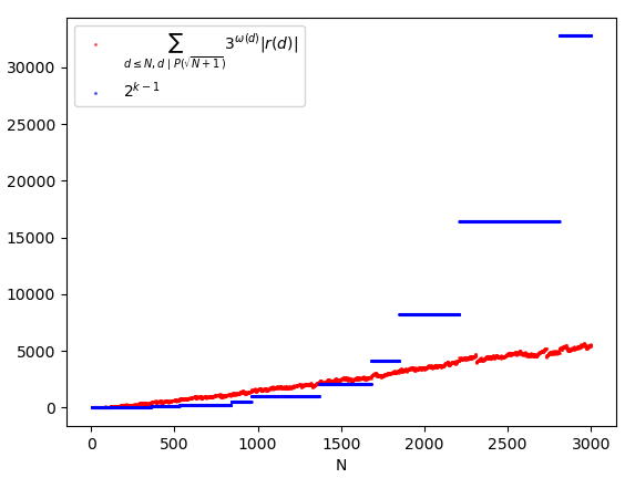
Taking into account that the true value is S(\{1, 2, \ldots, 100\}, \mathbb{P}, \sqrt{101}) = |\{p \mid 10 \lt p \leq 100\}| = 21, we certainly cannot say that we have approximated the function well! Furthermore, the margin of error of 60.58 that we obtained is much higher than what the approximation of the previous article would have, i.e. 2^{k-1} = 2^3 = 8 (where k = 4 because there are 4 primes less than or equal to \sqrt{100}).
Can we therefore conclude that Selberg’s sieve is a terrible overestimation? Certainly not. All this evidence concerns the single example taken into consideration, but what interests us most is always the asymptotic behavior. The error term of Selberg’s sieve continues to be greater than 2^{k-1} at least up to N = 1000:

However, if we extend our sample up to N = 3000, we notice that there is a reversal of trend in the error:
And if we continue up to N = 10,000, the trend is even more evident:

So, once again, it’s worth to remember that the examples must be taken for what they are, that is, individual cases. We should therefore not be discouraged if the results don’t seem promising, but we have to examine many examples in order to understand the asymptotic behavior of the functions we are studying (when it is not already known on a theoretical level).
Introduction to the proof
The proof of Selberg’s sieve is important because it applies a series of techniques that we can define as “smart”. In this article we’ll see the beginning of the proof, while in the next articles well delve deeper into some of its specific parts.
From here on the theory becomes more complex, with the risk of losing the perception of the practical meaning of the various steps, so we’ll carry on both the theory and a representative example in parallel. In particular, we’ll assume that the prime numbers used in the sieve are 3, that is P(z) = 2 \cdot 3 \cdot 5 (z could be any real number greater than 5 and less than or equal to 7; for now it’s not important to set a specific value).
Let’s start from Property C.2 (Sieve function with \mathcal{P} = \mathbb{P}, purely algebraic expression):
which is nothing other than the algebraic expression of the definition of sieve: the count of the elements of A coprime with P(z). We can rewrite the summation as follows:
which is equivalent to the previous expression, because we are counting 1 for the coprime elements with P(z) and 0 for all the others. But the function defined by cases that appears within the summation, by Property N.11 , can be expressed as a summation of the Möbius function:
So far we are still calculating the exact value of the sieve function. The idea of Selberg’s sieve consists in replacing the values of the function \mu(d) with real numbers \lambda_d, raising the sum to the square, for technical reasons which will be clear later. The Selberg approximation is therefore of the following type:
But Selberg’s sieve is an overestimation, so it must be:
How can we choose \lambda_ds such that this property is satisfied? It’s quite simple: just set \lambda_1 = 1, while the others \lambda_d can be any real numbers.
Why is (2) satisfied for \lambda_1 = 1, independently of the other \lambda_ds?
We can distinguish two cases:
- If \mathrm{GCD}(a, P(z)) = 1, the unique divisor d in common between a and P(z) is 1, so (3) reduces to:
\left( \lambda_1 \right)^2 \geq \mu(1)
But \mu(1) = 1, so it must be \left( \lambda_1 \right)^2 \geq 1, hence |\lambda_d| \geq 1. Since we want the smallest possible excess approximation (i.e. as close as possible to the real value), we choose \lambda_1 = 1 (the choice \lambda_1 = -1 would be been equivalent). Obviously in this case the other \lambda_ds can be any, since they do not appear in the previous inequality.
- If \mathrm{GCD}(a, P(z)) \gt 1, the right-hand side of (3) is 0 by Property N.11, so (2) reduces to:
\left( \sum_{d \mid \mathrm{GCD}(a, P(z))} \lambda_d \right)^2 \geq 0
But we know that the square of a real number is always greater than or equal to zero, so in this case (3) is satisfied whatever the values of \lambda_ds (including \lambda_1).
Considering both cases, we can therefore conclude that \lambda_1 must be 1 (otherwise the first case would not be satisfied), while the other \lambda_ds can be any, given that in neither case is there a constraint on them.
From (2) and (3) we can conclude:
At this point the proof is developed into three parts:
- the first part consists in writing the right part of formula (4) differently in order to achieve the form |A| T + R, where T represents the fraction of A elements remaining after applying the sieve, and R is the error term;
- the second part is the choice of the values of the constants \lambda_d which minimize the value of T (in order to have an estimate as close as possible to the real value) ;
- the third part consists in substituting the values of \lambda_ds within the error term R and carrying out the appropriate simplifications.
We’ll see the first part in the next paragraph and the other two parts in the next articles.
First part of the proof: the form |A| T + R
This part of the proof is divided into three steps: let’s look at them one at a time.
First step
The first step is as follows:
which is a consequence of the equality:
The notation is a bit complex, but the basic concept is simple; it is the same concept underlying the identity (a + b)^2 = (a + b)(a + b) = a \cdot a + a \cdot b + b \cdot a + b \cdot b (usually abbreviated to a^2 + 2ab + b^2). In essence, squaring a sum of n terms gives a sum of n^2 terms, containing all the possible products of two elements.
In our case, the number of elements of the squared summation is equal to the number of divisors of \mathrm{GCD}(a, P(z)), that is, it is equal to the number of common divisors between a and P(z) (remember that, by definition, every common divisor divides the greatest common divisor). For each of these common divisors d, the summation includes the corresponding constant \lambda_d. Let’s see an example.
Suppose that P(z) = 2 \cdot 3 \cdot 5. Then the divisors of P(z) are 1, 2, 3, 5, 6, 10, 15 and 30, consequently we’ll have the constants \lambda_1, \lambda_2, \lambda_3, \lambda_5, \lambda_6, \lambda_{10}, \lambda_{15} and \lambda_{30}. The summation \sum_{d \mid \mathrm{GCD}(a, P(z))} \lambda_d will therefore contain one or more of them, depending on which of the divisors of P(z) are also divisors of a. To make this concept more evident, we can use the symbol
to indicate the complete summation \lambda_1 + \lambda_2 + \lambda_3 + \lambda_5 + \lambda_6 + \lambda_{10} + \lambda_{15} + \lambda_{30} = \sum_{d \mid 30} \lambda_d, replacing the missing constants with an asterisk in the other summations. For example, if a = 1, the only common divisor with P(z) is 1 itself, then we’ll use the notation:
If a = 5, \mathrm{GCD}(a, P(z)) = 5 and the common divisors are 1 and 5, so we’ll use the notation:
If a = 12, \mathrm{GCD}(a, P(z)) = 6 and the common divisors are 1, 2, 3 and 6, so we’ll use the notation:
and so on.
For a = 6 the summation is the same as the one for a = 12, since the greatest common divisor with P(z) = 30 is 6 in both cases and therefore the common divisors with P(z) are the same too, i.e. 1, 2, 3 and 6.
This notation can easily be extended to represent the square of the summation \sum_{d \mid \mathrm{GCD}(a, P(z))} \lambda_d. We can in fact construct the following multiplicative table:
| \cdot | \mathbf{\lambda_1} | \mathbf{\lambda_2} | \mathbf{\lambda_3} | \mathbf{\lambda_6} | \mathbf{\lambda_{10}} | \mathbf{\lambda_{15}} | \mathbf{\lambda_{30}} |
|---|---|---|---|---|---|---|---|
| \mathbf{\lambda_1} | \lambda_1 \lambda_1 | \lambda_1 \lambda_2 | \lambda_1 \lambda_3 | \lambda_1 \lambda_6 | \lambda_1 \lambda_{10} | \lambda_1 \lambda_{15} | \lambda_1 \lambda_{30} |
| \mathbf{\lambda_2} | \lambda_2 \lambda_1 | \lambda_2 \lambda_2 | \lambda_2 \lambda_3 | \lambda_2 \lambda_6 | \lambda_2 \lambda_{10} | \lambda_2 \lambda_{15} | \lambda_2 \lambda_{30} |
| \mathbf{\lambda_3} | \lambda_3 \lambda_1 | \lambda_3 \lambda_2 | \lambda_3 \lambda_3 | \lambda_3 \lambda_6 | \lambda_3 \lambda_{10} | \lambda_3 \lambda_{15} | \lambda_3 \lambda_{30} |
| \mathbf{\lambda_5} | \lambda_5 \lambda_1 | \lambda_5 \lambda_2 | \lambda_5 \lambda_3 | \lambda_5 \lambda_6 | \lambda_5 \lambda_{10} | \lambda_5 \lambda_{15} | \lambda_5 \lambda_{30} |
| \mathbf{\lambda_6} | \lambda_6 \lambda_1 | \lambda_6 \lambda_2 | \lambda_6 \lambda_3 | \lambda_6 \lambda_6 | \lambda_6 \lambda_{10} | \lambda_6 \lambda_{15} | \lambda_6 \lambda_{30} |
| \mathbf{\lambda_{10}} | \lambda_{10} \lambda_1 | \lambda_{10} \lambda_2 | \lambda_{10} \lambda_3 | \lambda_{10} \lambda_6 | \lambda_{10} \lambda_{10} | \lambda_{10} \lambda_{15} | \lambda_{10} \lambda_{30} |
| \mathbf{\lambda_{15}} | \lambda_{15} \lambda_1 | \lambda_{15} \lambda_2 | \lambda_{15} \lambda_3 | \lambda_{15} \lambda_6 | \lambda_{15} \lambda_{10} | \lambda_{15} \lambda_{15} | \lambda_{15} \lambda_{30} |
| \mathbf{\lambda_{30}} | \lambda_{30} \lambda_1 | \lambda_{30} \lambda_2 | \lambda_{30} \lambda_3 | \lambda_{30} \lambda_6 | \lambda_{30} \lambda_{10} | \lambda_{30} \lambda_{15} | \lambda_{30} \lambda_{30} |
As you can easily verify, the sum of the table elements (excluding headers) is the result of the (\lambda_1 + \lambda_2 + \lambda_3 + \lambda_5 + \lambda_6 + \lambda_{10} + \lambda_{15} + \lambda_{30})^2 = \left( \sum_{d \mid 30} \lambda_d \right)^2 = \sum_{d_1 \mid 30} \sum_{d_2 \mid 30} \lambda_{d_1} \lambda_{d_2}. We can therefore represent the double summation with the symbol:
In the squares of the other summations we’ll replace the missing terms with asterisks. For example, for a = 1:
For a = 5:
For a = 6 or a = 12:
Second step
The second step is as follows:
In the previous step we regarded the double summation
as the sum of the elements of a matrix having elements of the type \lambda_{d_1} \lambda_{d_2}, where d_1 and d_2 are common divisors between a and P(z). So, if we fix a value of a, we’ll obtain a certain matrix, which we’ll call M_{\mathrm{GCD}(a, P(z))}, having rows and columns numbered with the divisors of P(z), in which only the cells the row and column of which are divisors of \mathrm{GCD}(a, P(z)) are filled.
Let’s see what are the matrices M_{\mathrm{GCD}(a, P(z))}, assuming that P(z) = 2 \cdot 3 \cdot 5 = 30. We’ll have a different matrix for each possible value of \mathrm{GCD}(a, 30). But the possible values of \mathrm{GCD}(a, 30) are no other than the divisors of 30 (the explanation is simple: being \mathrm{GCD}(a, 30) a common divisor between a and 30, in particular it is a divisor of 30; furthermore every divisor of 30 is the greatest common divisor between itself and 30, therefore it is one of the possible values of \mathrm{GCD}(a, 30)). Since 30 is the product of 2, 3 and 5, the divisors of 30 are the product of zero or more prime factors chosen from the set \{2, 3, 5\}, i.e. 1 (product of 0 prime factors), 2, 3 and 5 (products of 1 prime factor), 6, 10 and 15 (product of two prime factors), and 30 (product of all three prime factors). We’ll therefore have the following 8 cases:
- \mathrm{GCD}(a, 30) = 1 (a is not divisible neither by 2, nor by 3, nor by 5). In this case the only common divisor is 1, so the only full cell is the one with row 1 and column 1:
M_1 := \left( \begin{matrix} \lambda_1 \lambda_1 & * & * & * & * & * & * & * \\ * & * & * & * & * & * & * & * \\ * & * & * & * & * & * & * & * \\ * & * & * & * & * & * & * & * \\ * & * & * & * & * & * & * & * \\ * & * & * & * & * & * & * & * \\ * & * & * & * & * & * & * & * \\ * & * & * & * & * & * & * & * \end{matrix} \right)
- \mathrm{GCD}(a, 30) = 2 (a is divisible by 2, it is not divisible by either 3 or 5). In this case the filled cells are those the row and column of which are divisors of 2, i.e. 1 or 2:
M_2 := \left( \begin{matrix} \lambda_1 \lambda_1 & \lambda_1 \lambda_2 & * & * & * & * & * & * \\ \lambda_2 \lambda_1 & \lambda_2 \lambda_2 & * & * & * & * & * & * \\ * & * & * & * & * & * & * & * \\ * & * & * & * & * & * & * & * \\ * & * & * & * & * & * & * & * \\ * & * & * & * & * & * & * & * \\ * & * & * & * & * & * & * & * \\ * & * & * & * & * & * & * & * \end{matrix}\right)
- \mathrm{GCD}(a, 30) = 3 (a is divisible by 3, it is not divisible by either 2 or 5). In this case the full cells are those the row and column of which are divisors of 3, i.e. 1 or 3:
M_3 := \left( \begin{matrix} \lambda_1 \lambda_1 & * & \lambda_1 \lambda_3 & * & * & * & * & * \\ * & * & * & * & * & * & * & * \\ \lambda_3 \lambda_1 & * & \lambda_3 \lambda_3 & * & * & * & * & * \\ * & * & * & * & * & * & * & * \\ * & * & * & * & * & * & * & * \\ * & * & * & * & * & * & * & * \\ * & * & * & * & * & * & * & * \\ * & * & * & * & * & * & * & * \end{matrix}\right)
- \mathrm{GCD}(a, 30) = 5 (a is divisible by 5, it is not divisible by either 2 or 3). In this case the filled cells are those the row and column of which are divisors of 5, i.e. 1 or 5:
M_5 := \left( \begin{matrix} \lambda_1 \lambda_1 & * & * & \lambda_1 \lambda_5 & * & * & * & * \\ * & * & * & * & * & * & * & * \\ * & * & * & * & * & * & * & * \\ \lambda_5 \lambda_1 & * & * & \lambda_5 \lambda_5 & * & * & * & * \\ * & * & * & * & * & * & * & * \\ * & * & * & * & * & * & * & * \\ * & * & * & * & * & * & * & * \\ * & * & * & * & * & * & * & * \end{matrix}\right)
- \mathrm{GCD}(a, 30) = 6 (a is divisible by 2 and 3, but not by 5). In this case the filled cells are those the row and column of which are divisors of 6, i.e. 1, 2, 3 or 6:
M_6 := \left( \begin{matrix} \lambda_1 \lambda_1 & \lambda_1 \lambda_2 & \lambda_1 \lambda_3 & * & \lambda_1 \lambda_6 & * & * & * \\ \lambda_2 \lambda_1 & \lambda_2 \lambda_2 & \lambda_2 \lambda_3 & * & \lambda_2 \lambda_6 & * & * & * \\ \lambda_3 \lambda_1 & \lambda_3 \lambda_2 & \lambda_3 \lambda_3 & * & \lambda_3 \lambda_6 & * & * & * \\ * & * & * & * & * & * & * & * \\ \lambda_6 \lambda_1 & \lambda_6 \lambda_2 & \lambda_6 \lambda_3 & * & \lambda_6 \lambda_6 & * & * & * \\ * & * & * & * & * & * & * & * \\ * & * & * & * & * & * & * & * \\ * & * & * & * & * & * & * & * \end{matrix}\right)
- \mathrm{GCD}(a, 30) = 10 (a is divisible by 2 and 5, but not by 3). In this case the filled cells are those the row and column of which are divisors of 10, i.e. 1, 2, 5 or 10:
M_{10} := \left(\begin{matrix} \lambda_1 \lambda_1 & \lambda_1 \lambda_2 & * & \lambda_1 \lambda_5 & * & \lambda_1 \lambda_{10} & * & * \\ \lambda_2 \lambda_1 & \lambda_2 \lambda_2 & * & \lambda_2 \lambda_5 & * & \lambda_2 \lambda_{10} & * & * \\ \lambda_3 \lambda_1 & \lambda_3 \lambda_2 & * & \lambda_3 \lambda_5 & * & \lambda_3 \lambda_{10} & * & * \\ * & * & * & * & * & * & * & * \\ * & * & * & * & * & * & * & * \\ \lambda_{10} \lambda_1 & \lambda_{10} \lambda_2 & * & \lambda_{10} \lambda_5 & * & \lambda_{10} & * & * \\ * & * & * & * & * & * & * & * \\ * & * & * & * & * & * & * & * \end{matrix}\right)
- \mathrm{GCD}(a, 30) = 15 (a is divisible by 3 and 5, but not by 2). In this case the filled cells are those the row and column of which are divisors of 15, i.e. 1, 3, 5 or 15:
M_{15} := \left( \begin{matrix} \lambda_1 \lambda_1 & * & \lambda_1 \lambda_3 & \lambda_1 \lambda_5 & * & * & \lambda_1 \lambda_{15} & * \\ * & * & * & * & * & * & * & * \\ \lambda_3 \lambda_1 & * & \lambda_3 \lambda_3 & \lambda_3 \lambda_5 & * & * & \lambda_3 \lambda_{15} & * \\ * & * & * & * & * & * & * & * \\ * & * & * & * & * & * & * & * \\ * & * & * & * & * & * & * & * \\ \lambda_{15} \lambda_1 & * & \lambda_{15} \lambda_3 & \lambda_{15} \lambda_5 & * & * & \lambda_{15} \lambda_{15} & * \\ * & * & * & * & * & * & * & * \end{matrix}\right)
- \mathrm{GCD}(a, 30) = 30 (a is divisible by 2, by 3 and by 5). In this case we’ll have the complete matrix, because all the rows and all the columns are divisors of 30:
M_{30} := \left( \begin{matrix} \lambda_1 \lambda_1 & \lambda_1 \lambda_2 & \lambda_1 \lambda_3 & \lambda_1 \lambda_5 & \lambda_1 \lambda_6 & \lambda_1 \lambda_{10} & \lambda_1 \lambda_{15} & \lambda_1 \lambda_{30} \\ \lambda_2 \lambda_1 & \lambda_2 \lambda_2 & \lambda_2 \lambda_3 & \lambda_2 \lambda_5 & \lambda_2 \lambda_6 & \lambda_2 \lambda_{10} & \lambda_2 \lambda_{15} & \lambda_2 \lambda_{30} \\ \lambda_3 \lambda_1 & \lambda_3 \lambda_2 & \lambda_3 \lambda_3 & \lambda_3 \lambda_5 & \lambda_3 \lambda_6 & \lambda_3 \lambda_{10} & \lambda_3 \lambda_{15} & \lambda_3 \lambda_{30} \\ \lambda_5 \lambda_1 & \lambda_5 \lambda_2 & \lambda_5 \lambda_3 & \lambda_5 \lambda_5 & \lambda_5 \lambda_6 & \lambda_5 \lambda_{10} & \lambda_5 \lambda_{15} & \lambda_5 \lambda_{30} \\ \lambda_6 \lambda_1 & \lambda_6 \lambda_2 & \lambda_6 \lambda_3 & \lambda_6 \lambda_5 & \lambda_6 \lambda_6 & \lambda_6 \lambda_{10} & \lambda_6 \lambda_{15} & \lambda_6 \lambda_{30} \\ \lambda_{10} \lambda_1 & \lambda_{10} \lambda_2 & \lambda_{10} \lambda_3 & \lambda_{10} \lambda_5 & \lambda_{10} \lambda_6 & \lambda_{10} \lambda_{10} & \lambda_{10} \lambda_{15} & \lambda_{10} \lambda_{30} \\ \lambda_{15} \lambda_1 & \lambda_{15} \lambda_2 & \lambda_{15} \lambda_3 & \lambda_{15} \lambda_5 & \lambda_{15} \lambda_6 & \lambda_{15} \lambda_{10} & \lambda_{15} \lambda_{15} & \lambda_{15} \lambda_{30} \\ \lambda_{30} \lambda_1 & \lambda_{30} \lambda_2 & \lambda_{30} \lambda_3 & \lambda_{30} \lambda_5 & \lambda_{30} \lambda_6 & \lambda_{30} \lambda_{10} & \lambda_{30} \lambda_{15} & \lambda_{30} \lambda_{30} \end{matrix}\right)
As it can be easily verified, the sum of the elements of the matrix M_d, for d \in \{1, 2, 3, 5, 6, 10, 15, 30\} , is:
Equation (5) tells us that we must add up the matrices of all as:
For a = 1, 2, 3, 4, 5, 6, 7, 8, 9, 10, \ldots, being respectively \mathrm{GCD}(a, 30) = 1, 2, 3, 2, 5, 6, 1, 2, 3, 10, \ldots, summation (b) becomes:
As we have seen, all the elements of the matrices M_{\mathrm{GCD}(a, P(z))} are of the type \lambda_{d_1} \lambda_{d_2}, with d_1, d_2 divisors of P(z); there are no elements of different types. This observation suggests an alternative way of adding up all the matrices: instead of starting from the various as and adding the matrices one at a time, we can start from the possible elements and multiply each of them by the number of matrices in which it appears:
This way we are still adding all the elements of all the matrices, because we are considering all the possible elements and each of them is multiplied by the number of matrices in which it is present. So the final result must be the same as before:
It is now a question of establishing, given two divisors of P(z), d_1 and d_2, in how many matrices the element \lambda_{d_1} \lambda_{d_2}. It might seem a complicated question, but the answer is very simple:
That is, the element \lambda_{d_1} \lambda_{d_2} appears in all and only the matrices M_{\mathrm{GCD}(a, P(z))} where a is a multiple of both d_1 and d_2. Let’s see why:
- If a is a multiple of both d_1 and d_2, being also by hypothesis P(z) multiple of both, d_1 and d_2 are common divisors between a and P(z), therefore they divide \mathrm{GCD}(a, P(z)). But the elements of the matrix M_{\mathrm{GCD}(a, P(z))} are precisely those the row and column numbers of which are the divisors of \mathrm{GCD}(a, P(z)); one of them will therefore be \lambda_{d_1} \lambda_{d_2}. This proves the leftward implication of e).
- The previous reasoning can be repeated in reverse: if the element \lambda_{d_1} \lambda_{d_2} is present in a matrix M_{\mathrm{GCD}(a , P(z))}, it means that d_1 and d_2 divide \mathrm{GCD}(a, P(z)); but the latter is in turn a divisor of a, so d_1 and d_2 divide a. This proves the rightward implication.
Supposing again that P(z) = 2 \cdot 3 \cdot 5 = 30, let’s examine three cases:
- d_1 = d_2 = 1.
In this case any a is a multiple of both d_1 and d_2. So, by (e), the element \lambda_{d_1} \lambda_{d_2} appears in all matrices. We can find confirmation in the first example: in all 8 possible matrices, the top left cell is always filled, and it contains the element \lambda_1 \lambda_1. - d_1 = d_2 = 2.
In this case, by (e), the element \lambda_{d_1} \lambda_{d_2} appears in all and only the matrices M_{\mathrm{GCD}(a, 30)} where a is even. Let’s consider the summation (c): the matrices we find when a = 2, 4, 6, 8, 10 are respectively M_2, M_2, M_6, M_2, M_{10} and they, as it can be verified in the first example, all contain the element \lambda_2 \lambda_2; on the contrary, the matrices we find when a = 1, 3, 5, 7, 9 are respectively M_1, M_3, M_5, M_1, M_3, and none of them contains the element \lambda_2 \lambda_2. - d_1 = 2, d_2 = 3.
In this case, by (e), the element \lambda_{d_1} \lambda_{d_2} appears in all and only the matrices M_{\mathrm{GCD}(a, 30)} where a is a multiple of 6. In the summation (c), the only value of a that is a multiple of 6 is 6 itself, and the corresponding matrix, the sixth of the summation, is M_6. As it can easily be verified, M_6 is the only one among the matrices of summation (c) that contains the element \lambda_2 \lambda_3. If we continued the summation, we would obtain the same matrix also for a = 12, 18, 24, because the greatest common divisor between these numbers and 30 is always 6. Moreover, for a = 30 we would have the matrix M_{30}, which obviously also contains the element, being the complete one.
Now we can draw our conclusions:
where the last step uses the notation introduced in the statement of Selberg’s sieve (Theorem C.4).
Substituting into (d), we’ll obtain (6).
Third step
The third step is as follows:
The purpose of this step is to highlight |A|. Using the notations of Theorem C.4, we’ll have that:
In this equality there are three important quantities:
- |A_d| is the number of multiples of d in A; since A contains all positive integers from 1 to a certain number, |A_d| is equal to \left\lfloor \frac{|A|}{d} \right\rfloor, the integer part of dividing the number of elements of A (which coincides with its largest element) by d.
- \frac{|A|}{d} is an approximation of the number of multiples of d in A: instead of taking the integer part of the division, here we are taking the fraction as it is.
- r(d) is the difference between the previous quantities, i.e. it indicates how much we are wrong when approximating |A_d| with \frac{|A|}{d}. Perhaps a little counterintuitively, if r(d) \neq 0 the sign is negative because |A_d| \leq \frac{|A|}{d}, since the integer part of a fraction is always less than or equal to the fraction itself. However, the sign has little importance, because what is of most interest is the absolute value of r(d).
If A = \{1, 2, 3, \ldots, 100\} and d = 3, we’ll have that:
- |A_3| = \left\lfloor \frac{|A|}{3} \right\rfloor = \left\lfloor \frac{100}{3} \right\rfloor = 33, because there are 33 multiples of 3 less than or equal to 100;
- \frac{|A|}{3} = \frac{100}{3} = 33.333\ldots is an approximation of the previous number, without the integer part;
- r(3) = |A_3| - \frac{|A|}{3} = 33 - \frac{100}{3} = \frac{99 - 100}{3} = -\frac{1}{3} = -0.333\ldots is the difference between the previous quantities, with a negative sign.
From (f), substituting d := \mathrm{lcm}(d_1 d_2), we’ll obtain:
hence:
This step allows us to obtain the form |A| T + R, by putting:
So, combining formulas from (4) to (7), we’ll obtain:
From this inequality it is clear that T is the quantity to be minimized in order to obtain an estimate |A| T as close as possible to the exact value, while R represents the error term.