Selberg’s sieve: study of the parameters λ

Prerequisites:

As we have seen, some parameters \lambda_d appear in the Selberg’s sieve formula, which are used both in the estimation of the sieve function and in the related error term. In this article we’ll calculate these parameters in order to obtain the lowest possible estimate.

In the previous article we saw that, if A is a finite set of natural numbers, z \gt 1 is a real number and P(z) is the product of the prime numbers smaller than z, then:

S(A, \mathbb{P}, z) \leq |A| T + R

where:

T := \sum_{d_1, d_2 \mid P(z)} \frac{\lambda_{d_1} \lambda_{d_2}}{\mathrm{lcm}(d_1, d_2)} \tag{1}
R := \sum_{d_1, d_2 \mid P(z)} \lambda_{d_1} \lambda_{d_2} r(\mathrm{lcm}(d_1, d_2)) \tag{2}

Recall that the \lambda_ds (where d represents a divisor of P(z)) are real numbers that can be chosen as desired, with the only constraint that \lambda_1 = 1. In this article we’ll focus on formula (1) and we’ll calculate what values the \lambda_d should have to make the T summation as low as possible. The calculation can be structured in the steps that we’ll analyze below.

Step 1: from least common multiple to greatest common divisor

The least common multiple is a bit annoying in number theory, because almost all formulas operate in terms of divisors rather than multiples: it is a purely conventional choice which, however, should be adapted to. We’ll transform the least common multiple into the greatest common divisor using the well-known property \mathrm{lcm}(d_1, d_2) = \frac{d_1 d_2}{\mathrm{GCD}(d_1, d_2)}, applying which from formula (1) we’ll obtain:

T = \sum_{d_1, d_2 \mid P(z)} \frac{\lambda_{d_1} \lambda_{d_2}}{d_1 d_2} \mathrm{GCD}(d_1, d_2) \tag{3}

Step 2: introduction of the divisors of the greatest common divisor, using the Möbius inversion formula

Now we’ll introduce a further level of divisors using the Möbius inversion formula. Applying Property N.18 (including the Remark that follows it) with n := \mathrm{GCD}(d_1, d_2) and f := \mathrm{id} (identity function f(x) = x), we’ll get:

\mathrm{GCD}(d_1, d_2) = \sum_{d \mid \mathrm{GCD}(d_1, d_2)} \sum_{d ^{\prime} d^{\prime \prime} = d} \mu(d^{\prime}) d^{\prime \prime}

Now let’s define:

\phi(d) := \sum_{d^{\prime} d^{\prime \prime} = d} \mu(d^{\prime}) d^{\prime \prime}

From which:

\mathrm{GCD}(d_1, d_2) = \sum_{d \mid \mathrm{GCD}(d_1, d_2)} \phi(d)

Substituting into (3), we’ll have:

T = \sum_{d_1, d_2 \mid P(z)} \frac{\lambda_{d_1} \lambda_{d_2}}{d_1 d_2} \sum_{d \mid \mathrm{GCD}(d_1, d_2)} \phi(d)\tag{4}

Suppose that P(z) = 2 \cdot 3 \cdot 5 = 30 and we want to calculate the possible values of \phi(d). In this regard it must be noted that d is a divisor of \mathrm{GCD}(d_1, d_2), which in turn is a divisor of d_1 and d_2 which in turn are divisors of P(z); therefore, by transitivity, d is also a divisor of P(z). To make sure to compute all possible values, we’ll then compute \phi(d) for all divisors of 30:

\begin{aligned} \phi(1) & = \sum_{d^{\prime} d^{\prime \prime} = 1} \mu(d^{\prime}) d^{\prime \prime} = \mu(1) 1 = 1 \\ \phi(2) & = \sum_{d^{\prime} d^{\prime \prime} = 2} \mu(d^{\prime}) d^{\prime \prime} = \mu(1) 2 + \mu(2) 1 = 2 - 1 = 1 \\ \phi(3) & = \sum_{d^{\prime} d^{\prime \prime} = 3} \mu(d^{\prime}) d^{\prime \prime} = \mu(1) 3 + \mu(3) 1 = 3 - 1 = 2 \\ \phi(5) & = \sum_{d^{\prime} d^{\prime \prime} = 5} \mu(d^{\prime}) d^{\prime \prime} = \mu(1) 5 + \mu(5) 1 = 5 - 1 = 4 \\ \phi(6) &= \sum_{d^{\prime} d^{\prime \prime} = 6} \mu(d^{\prime}) d^{\prime \prime} = \mu(1) 6 + \mu(2) 3 + \mu(3) 2 + \mu(6) 1 = 6 - 3 - 2 + 1 = 2 \\ \phi(10) & = \sum_{d^{\prime} d^{\prime \prime} = 10} \mu(d^{\prime}) d^{\prime \prime} = \mu(1) 10 + \mu(2) 5 + \mu(5) 2 + \mu(10) 1 = 10 - 5 - 2 + 1 = 4 \\ \phi(15) & = \sum_{d^{\prime} d^{\prime \prime} = 15} \mu(d^{\prime}) d^{\prime \prime} = \mu(1) 15 + \mu(3) 5 + \mu(5) 3 + \mu(15) 1 = 15 - 5 - 3 + 1 = 8 \\ \phi(30) & = \sum_{d^{\prime} d^{\prime \prime} = 30} \mu(d^{\prime}) d^{\prime \prime} = \mu(1) 30 + \mu(2) 15 + \mu(3) 10 + \mu(5) 6 + \mu(6) 5 + \mu(10) 3 + \mu(15) 2 + \mu(30) 1 \\ & = 30 - 15 - 10 - 6 + 5 + 3 + 2 - 1 = 8 \end{aligned}

We have called \phi this function because, for the examples that interest us, it coincides with Euler’s function, which is usually denoted by the same symbol. The two functions coincide on all square-free numbers, i.e. the ones which are the product of distinct prime factors. This coincidence is quite surprising, given that the two functions are defined in two very different ways.

Step 3: Collect repeating \phi(d) values

In (4), we can observe that multiple pairs of integers d_1 and d_2, divisors of P(z), can have the same greatest common divisor; in this case the divisors d of the greatest common divisor will be the same, and therefore the values of \phi(d) of the internal summation will be repeated for each pair. For example, if P(z) = 2 \cdot 3 \cdot 5, the value \phi(2) will occur for both the pair (d_1, d_2) = (2, 2) and the pair (d_1, d_2) = (10, 6), because both pairs of numbers have a least common multiple equal to 2. More generally, \phi(2) will be repeated for all pairs (d_1, d_2) which have a multiple of 2 as their greatest common divisor, as can be seen from the internal summation by substituting d = 2.
Collecting these repeated \phi(d) values, we’ll obtain:

T = \sum_{d \mid P(z)} \phi(d) \sum_{\substack{d_1, d_2 \mid P(z) \\ d \mid \mathrm{GCD}(d_1, d_2)}} \frac{\lambda_{d_1} \lambda_{d_2}}{d_1 d_2} \tag{5}

Suppose that P(z) = 2 \cdot 3. Then formula (4) can be expanded as follows:

\begin{aligned} T & = \sum_{d_1, d_2 \mid 6} \frac{\lambda_{d_1} \lambda_{d_2}}{d_1 d_2} \sum_{d \mid \mathrm{GCD}(d_1, d_2)} \phi(d) \\ \\ & = \frac{\lambda_{1} \lambda_{1}}{1 \cdot 1} \sum_{d \mid \mathrm{GCD}(1, 1)} \phi(d) + \frac{\lambda_{1} \lambda_{2}}{1 \cdot 2} \sum_{d \mid \mathrm{GCD}(1, 2)} \phi(d) \frac{\lambda_{1} \lambda_{3}}{1 \cdot 3} \sum_{d \mid \mathrm{GCD}(1, 3)} \phi(d) + \frac{\lambda_{1} \lambda_{6}}{1 \cdot 6} \sum_{d \mid \mathrm{GCD}(1, 6)} \phi(d) \\ & + \frac{\lambda_{2} \lambda_{1}}{2 \cdot 1} \sum_{d \mid \mathrm{GCD}(2, 1)} \phi(d) + \frac{\lambda_{2} \lambda_{2}}{2 \cdot 2} \sum_{d \mid \mathrm{GCD}(2, 2)} \phi(d) \frac{\lambda_{2} \lambda_{3}}{2 \cdot 3} \sum_{d \mid \mathrm{GCD}(2, 3)} \phi(d) + \frac{\lambda_{2} \lambda_{6}}{2 \cdot 6} \sum_{d \mid \mathrm{GCD}(2, 6)} \phi(d) \\ & + \frac{\lambda_{3} \lambda_{1}}{3 \cdot 1} \sum_{d \mid \mathrm{GCD}(3, 1)} \phi(d) + \frac{\lambda_{3} \lambda_{2}}{3 \cdot 2} \sum_{d \mid \mathrm{GCD}(3, 2)} \phi(d) \frac{\lambda_{3} \lambda_{3}}{3 \cdot 3} \sum_{d \mid \mathrm{GCD}(3, 3)} \phi(d) + \frac{\lambda_{3} \lambda_{6}}{3 \cdot 6} \sum_{d \mid \mathrm{GCD}(3, 6)} \phi(d) \\ & + \frac{\lambda_{6} \lambda_{1}}{6 \cdot 1} \sum_{d \mid \mathrm{GCD}(6, 1)} \phi(d) + \frac{\lambda_{6} \lambda_{2}}{6 \cdot 2} \sum_{d \mid \mathrm{GCD}(6, 2)} \phi(d) \frac{\lambda_{6} \lambda_{3}}{6 \cdot 3} \sum_{d \mid \mathrm{GCD}(6, 3)} \phi(d) + \frac{\lambda_{6} \lambda_{6}}{6 \cdot 6} \sum_{d \mid \mathrm{GCD}(6, 6)} \phi(d) \\ \\ & = \frac{\lambda_{1} \lambda_{1}}{1 \cdot 1} \phi(1) + \frac{\lambda_{1} \lambda_{2}}{1 \cdot 2} \phi(1) + \frac{\lambda_{1} \lambda_{3}}{1 \cdot 3} \phi(1) + \frac{\lambda_{1} \lambda_{6}}{1 \cdot 6} \phi(1) \\ & + \frac{\lambda_{2} \lambda_{1}}{2 \cdot 1} \phi(1) + \frac{\lambda_{2} \lambda_{2}}{2 \cdot 2} (\phi(1) + \phi(2)) + \frac{\lambda_{2} \lambda_{3}}{2 \cdot 3} \phi(1) + \frac{\lambda_{2} \lambda_{6}}{2 \cdot 6} (\phi(1) + \phi(2)) \\ & + \frac{\lambda_{3} \lambda_{1}}{3 \cdot 1} \phi(1) + \frac{\lambda_{3} \lambda_{2}}{3 \cdot 2} \phi(1) + \frac{\lambda_{3} \lambda_{3}}{3 \cdot 3} (\phi(1) + \phi(3)) + \frac{\lambda_{3} \lambda_{6}}{3 \cdot 6} (\phi(1) + \phi(3)) \\ & + \frac{\lambda_{6} \lambda_{1}}{6 \cdot 1} \phi(1) + \frac{\lambda_{6} \lambda_{2}}{6 \cdot 2} (\phi(1) + \phi(2)) + \frac{\lambda_{6} \lambda_{3}}{6 \cdot 3} (\phi(1) + \phi(3)) + \frac{\lambda_{6} \lambda_{6}}{6 \cdot 6} (\phi (1) + \phi(2) + \phi(3) + \phi(6)) \end{aligned}

We can observe that \phi(1) is multiplied by all the terms \frac{\lambda_{d_1} \lambda_{d_2}}{d_1 d_2}, because 1 \mid \mathrm{GCD}(d_1, d_2) whatever d_1 and d_2 are, while, on the contrary, \phi(6) appears only once. Collecting \phi(1), \phi(2), \phi(3) and \phi(6), we’ll obtain:

\begin{aligned} & = \phi(1) \left(\frac{\lambda_{1} \lambda_{1}}{1 \cdot 1} + \frac{\lambda_{1} \lambda_{2}}{1 \cdot 2} + \frac{\lambda_{1} \lambda_{3}}{1 \cdot 3} + \frac{\lambda_{1} \lambda_{6}}{1 \cdot 6} + \frac{\lambda_{2} \lambda_{1}}{2 \cdot 1} + \frac{\lambda_{2} \lambda_{2}}{2 \cdot 2} + \ldots + \frac{\lambda_{6} \lambda_{6}}{6 \cdot 6} \right) \\ & + \phi(2) \left(\frac{\lambda_{2} \lambda_{2}}{2 \cdot 2} + \frac{\lambda_{2} \lambda_{6}}{2 \cdot 6} + \frac{\lambda_{6} \lambda_{2}}{6 \cdot 2} + \frac{\lambda_{6} \lambda_{6}}{6 \cdot 6} \right) \\ & + \phi(3) \left(\frac{\lambda_{3} \lambda_{3}}{3 \cdot 3} + \frac{\lambda_{3} \lambda_{6}}{3 \cdot 6} + \frac{\lambda_{6} \lambda_{3}}{6 \cdot 3} + \frac{\lambda_{6} \lambda_{6}}{6 \cdot 6} \right) \\ & + \phi(6) \cdot \frac{\lambda_{6} \lambda_{6}}{6 \cdot 6} \\ \\ & = \phi(1) \sum_{\substack{d_1, d_2 \mid 6 \\ 1 \mid \mathrm{GCD}(d_1, d_2)}} \frac{\lambda_{d_1} \lambda_{d_2}}{d_1 d_2} + \phi(2) \sum_{\substack{d_1, d_2 \mid 6 \\ 2 \mid \mathrm{GCD}(d_1, d_2)}} \frac{\lambda_{d_1} \lambda_{d_2}}{d_1 d_2} + \phi(3) \sum_{\substack{d_1, d_2 \mid 6 \\ 3 \mid \mathrm{GCD}(d_1, d_2)}} \frac{\lambda_{d_1} \lambda_{d_2}}{d_1 d_2} + \phi(6) \sum_{\substack{d_1, d_2 \mid 6 \\ 6 \mid \mathrm{GCD}(d_1, d_2)}} \frac{\lambda_{d_1} \lambda_{d_2}}{d_1 d_2} \\ \\ & = \sum_{d \mid 6} \phi(d) \sum_{\substack{d_1, d_2 \mid P(z) \\ d \mid \mathrm{GCD}(d_1, d_2)}} \frac{\lambda_{d_1} \lambda_{d_2}}{d_1 d_2} \end{aligned}

Step 4: Locate the square

The innermost summation of (5) can be rewritten as the square of a simpler summation:

\sum_{\substack{d_1, d_2 \mid P(z) \\ d \mid \mathrm{GCD}(d_1, d_2)}} \frac{\lambda_{d_1} \lambda_{d_2}}{d_1 d_2} = \left(\sum_{d \mid d^{\prime} \mid P(z)} \frac{\lambda_{d^{\prime}}}{d^{\prime}}\right)^2 \tag{6}

The reason is that the condition d \mid \mathrm{GCD}(d_1, d_2) is equivalent to d \mid d_1 \land d \mid d_2, where we used the logical \land symbol to indicate that both conditions must be satisfied. In fact, by definition of greatest common divisor, all the divisors of the greatest common divisor between two numbers divide the numbers themselves and, vice versa, two numbers that divide them both are common divisors, therefore they are divisors of the greatest common divisor. So the left part of (6) can be rewritten as:

\sum_{\substack{d_1, d_2 \mid P(z) \\ d \mid d_1 \land d \mid d_2}} \frac{\lambda_{d_1} \lambda_{d_2}}{d_1 d_2}

which in turn can be written differently as follows:

\sum_{\substack{d \mid d_1 \mid P(z) \\ d \mid d_2 \mid P(z)}} \frac{\lambda_{d_1} \lambda_{d_2}}{d_1 d_2}

From this last summation we can obtain the right part of (6) using the same considerations as the “first step” (formula 5) of the previous article.

Let’s take the previous example again, where P(z) = 2 \cdot 3 and therefore d \mid P(z) \Leftrightarrow d \mid 6 \Leftrightarrow d \in \{1, 2, 3, 6\}. Let’s analyze the individual cases.

For d = 6 we’ll have that:

\sum_{\substack{d_1, d_2 \mid P(z) \\ d \mid \mathrm{GCD}(d_1, d_2)}} \frac{\lambda_{d_1} \lambda_{d_2}}{d_1 d_2} = \sum_{\substack{d_1, d_2 \mid 6 \\ 6 \mid \mathrm{GCD}(d_1, d_2)}} \frac{\lambda_{d_1} \lambda_{d_2}}{d_1 d_2}

From the condition 6 \mid \mathrm{GCD}(d_1, d_2) it follows that d_1 and d_2 are multiples of 6, but by the condition d_1, d_2 \mid 6 they divide 6, so it must be d_1 = d_2 = 6. So:

\begin{aligned} \sum_{\substack{d_1, d_2 \mid 6 \\ 6 \mid \mathrm{GCD}(d_1, d_2)}} \frac{\lambda_{d_1} \lambda_{d_2}}{d_1 d_2} = \sum_{d_1 = d_2 = 6} \frac{\lambda_{d_1} \lambda_{d_2}}{d_1 d_2} & = \\ \frac{\lambda_{6} \lambda_{6}}{6 \cdot 6} & = \\ \left(\frac{\lambda_6}{6} \right)^2 = \left(\sum_{d^{\prime} = 6} \frac{\lambda_{d^{\prime}}}{d^{\prime}}\right)^2 & = \\ \left(\sum_{6 \mid d ^{\prime} \mid 6} \frac{\lambda_{d^{\prime}}}{d^{\prime}}\right)^2 = \left(\sum_{d \mid d^{\prime} \mid P(z)} \frac{\lambda_{d^{\prime}}}{d^{\prime}}\right)^2 \end{aligned} \tag{a}

For d = 3 we’ll have that:

\sum_{\substack{d_1, d_2 \mid P(z) \\ d \mid \mathrm{GCD}(d_1, d_2)}} \frac{\lambda_{d_1} \lambda_{d_2}}{d_1 d_2} = \sum_{\substack{d_1, d_2 \mid 6 \\ 3 \mid \mathrm{GCD}(d_1, d_2)}} \frac{\lambda_{d_1} \lambda_{d_2}}{d_1 d_2}

From the condition 3 \mid \mathrm{GCD}(d_1, d_2) it follows that d_1 and d_2 are multiples of 3, but by the condition d_1, d_2 \mid 6 they divide 6, so each of them can be either 3 or 6. So:

\begin{aligned} \sum_{\substack{d_1, d_2 \mid 6 \\ 3 \mid \mathrm{GCD}(d_1, d_2)}} \frac{\lambda_{d_1} \lambda_{d_2}}{d_1 d_2} = \sum_{\substack{d_1 \in \{3, 6\} \\ d_2 \in \{3, 6\}}} \frac{\lambda_{d_1} \lambda_{d_2}}{d_1 d_2} & = \\ \frac{\lambda_{3} \lambda_{3}}{3 \cdot 3} + \frac{\lambda_{3} \lambda_{6}}{3 \cdot 6} + \frac{\lambda_{6} \lambda_{3}}{6 \cdot 3} + \frac{\lambda_{6} \lambda_{6}}{6 \cdot 6} & = \\ \left(\frac{\lambda_3}{3} + \frac{\lambda_6}{6} \right)^2 & = \\ \left(\sum_{d^{\prime} \in \{3, 6\}} \frac{\lambda_{d^{\prime}}}{d^{\prime}}\right)^2 = \left(\sum_{3 \mid d^{\prime} \mid 6} \frac{\lambda_{d^{\prime}}}{d^{\prime}}\right)^2 = \left(\sum_{d \mid d^{\prime} \mid P(z)} \frac{\lambda_{d^{\prime}}}{d^{\prime}}\right)^2 \end{aligned} \tag{b}

The case of d = 2 is analogous to that of d = 3, so let’s see directly what happens when d = 1:

\sum_{\substack{d_1, d_2 \mid P(z) \\ d \mid \mathrm{GCD}(d_1, d_2)}} \frac{\lambda_{d_1} \lambda_{d_2}}{d_1 d_2} = \sum_{\substack{d_1, d_2 \mid 6 \\ 1 \mid \mathrm{GCD}(d_1, d_2)}} \frac{\lambda_{d_1} \lambda_{d_2}}{d_1 d_2}

The condition 1 \mid \mathrm{GCD}(d_1, d_2) is always true, so this condition does not impose any further restrictions on d_1 and d_2, which according to the condition d_1, d_2 \mid 6 can be 1, 2, 3 or 6. So:

\begin{aligned} \sum_{\substack{d_1, d_2 \mid 6 \\ 1 \mid \mathrm{GCD}(d_1, d_2)}} \frac{\lambda_{d_1} \lambda_{d_2}}{d_1 d_2} = \sum_{\substack{d_1 \in \{1, 2, 3, 6\} \\ d_2 \in \{1, 2, 3, 6\}}} \frac{\lambda_{d_1} \lambda_{d_2}}{d_1 d_2} & = \\ \frac{\lambda_{1} \lambda_{1}}{1 \cdot 1} + \frac{\lambda_{1} \lambda_{2}}{1 \cdot 2} + \frac{\lambda_{1} \lambda_{3}}{1 \cdot 3} + \frac{\lambda_{1} \lambda_{6}}{1 \cdot 6} + \frac{\lambda_{2} \lambda_{1}}{2 \cdot 1} + \frac{\lambda_{2} \lambda_{2}}{2 \cdot 2} + \ldots + \frac{\lambda_{6} \lambda_{6}}{6 \cdot 6} & = \\ \left(\frac{\lambda_1}{1} + \frac{\lambda_2}{2} + \frac{\lambda_3}{3} + \frac{\lambda_6}{6} \right)^2 & = \\ \left(\sum_{d^{\prime} \in \{1, 2, 3, 6\}} \frac{\lambda_{d^{\prime}}}{d^{\prime}}\right)^2 = \left(\sum_{1 \mid d^{\prime} \mid 6} \frac{\lambda_{d^{\prime}}}{d^{\prime}}\right)^2 = \left(\sum_{d \mid d^{\prime} \mid P(z)} \frac{\lambda_{d^{\prime}}}{d^{\prime}}\right)^2 \end{aligned} \tag{c}

It can be observed that the summations (a), (b) and (c) are those that multiply respectively \phi(6), \phi(3) and \phi(1) in the previous example.

Substituting (6) into (5), we’ll obtain:

T = \sum_{d \mid P(z)} \phi(d) \left(\sum_{d \mid d^{\prime} \mid P(z)} \frac{\lambda_{d^{\prime}}}{d^{\prime}}\right)^2 \tag{7}

Step 5: introduce the new variable w_d

Now we can simplify formula (7) by putting:

w_d := \sum_{d \mid d^{\prime} \mid P(z)} \frac{\lambda_{d^{\prime}}}{d^{\prime}} \tag{8}

hence:

T = \sum_{d \mid P(z)} \phi(d) w_d^2 \tag{9}

We need such an expression of T in order to minimize it; in fact we can proceed in two phases:

  1. Find the values of w_d that minimize T in formula (9)
  2. Calculate the values of \lambda_d starting from the values of w_d, using (8)

These will be the next steps.

Let’s look at formula (8) more explicitly, assuming that P(z) = 2 \cdot 3 \cdot 5. The variable d, as it can be seen from formula (7), is a divisor of P(z), therefore the possible w_d are w_1, w_2, w_3, w_5, w_6, w_{10}, w_{15}, w_{30}. Let’s look at them one at a time:

\begin{aligned} w_1 &= \sum_{1 \mid d^{\prime} \mid 30} \frac{\lambda_{d^{\prime}}}{d^{\prime}} & = \sum_{d^{\prime} \in \{1, 2, 3, 5, 6, 10, 15, 30\}} \frac{\lambda_{d^{\prime}}}{d^{\prime}} & = \frac{\lambda_1}{1} + \frac{\lambda_2}{2} + \frac{\lambda_3}{3} + \frac{\lambda_5}{5} + \frac{\lambda_6}{6} + \frac{\lambda_{10}}{10} + \frac{\lambda_{15}}{15} + \frac{\lambda_{30}}{30} \\ w_2 & = \sum_{2 \mid d^{\prime} \mid 30} \frac{\lambda_{d^{\prime}}}{d^{\prime}} & = \sum_{d^{\prime} \in \{2, 6, 10, 30\}} \frac{\lambda_{d^{\prime}}}{d^{\prime}} & = \frac{\lambda_2}{2} + \frac{\lambda_6}{6} + \frac{\lambda_{10}}{10} + \frac{\lambda_{30}}{30} \\ w_3 & = \sum_{3 \mid d^{\prime} \mid 30} \frac{\lambda_{d^{\prime}}}{d^{\prime}} & = \sum_{d^{\prime} \in \{3, 6, 15, 30\}} \frac{\lambda_{d^{\prime}}}{d^{\prime}} & = \frac{\lambda_3}{3} + \frac{\lambda_6}{6} + \frac{\lambda_{15}}{15} + \frac{\lambda_{30}}{30} \\ w_5 & = \sum_{5 \mid d^{\prime} \mid 30} \frac{\lambda_{d^{\prime}}}{d^{\prime}} & = \sum_{d^{\prime} \in \{5, 10, 15, 30\}} \frac{\lambda_{d^{\prime}}}{d^{\prime}} & = \frac{\lambda_5}{5} + \frac{\lambda_{10}}{10} + \frac{\lambda_{15}}{15} + \frac{\lambda_{30}}{30} \\ w_6 & = \sum_{6 \mid d^{\prime} \mid 30} \frac{\lambda_{d^{\prime}}}{d^{\prime}} & = \sum_{d^{\prime} \in \{6, 30\}} \frac{\lambda_{d^{\prime}}}{d^{\prime}} & = \frac{\lambda_6}{6} + \frac{\lambda_{30}}{30} \\ w_{10} & = \sum_{10 \mid d^{\prime} \mid 30} \frac{\lambda_{d^{\prime}}}{d^{\prime}} & = \sum_{d^{\prime} \in \{10, 30\}} \frac{\lambda_{d^{\prime}}}{d^{\prime}} & = \frac{\lambda_{10}}{10} + \frac{\lambda_{30}}{30} \\ w_{15} & = \sum_{15 \mid d^{\prime} \mid 30} \frac{\lambda_{d^{\prime}}}{d^{\prime}} & = \sum_{d^{\prime} \in \{15, 30\}} \frac{\lambda_{d^{\prime}}}{d^{\prime}} & = \frac{\lambda_{15}}{15} + \frac{\lambda_{30}}{30} \\ w_{30} & = \sum_{30 \mid d^{\prime} \mid 30} \frac{\lambda_{d^{\prime}}}{d^{\prime}} & = \sum_{d^{\prime} \in \{30\}} \frac{\lambda_{d^{\prime}}}{d^{\prime}} & = \frac{\lambda_{30}}{30} \end{aligned}

Step 6: calculate \lambda_d starting from w_d

For reasons that will become clear shortly, let’s analyze the two remaining steps in reverse order, starting with the second. So let’s ask ourselves: how can we calculate the values of \lambda_d, once we have calculated those of w_d?
Let’s see an example.

As we saw in the previous example, formula (8) corresponds to the following system of equations:

\begin{cases} w_1 & = \frac{\lambda_1}{1} + \frac{\lambda_2}{2} + \frac{\lambda_3}{3} + \frac{\lambda_5}{5} + \frac{\lambda_6}{6} + \frac{\lambda_{10}}{10} + \frac{\lambda_{15}}{15} + \frac{\lambda_{30}}{30} \\ w_2 &= \frac{\lambda_2}{2} + \frac{\lambda_6}{6} + \frac{\lambda_{10}}{10} + \frac{\lambda_{30}}{30} \\ w_3 &= \frac{\lambda_3}{3} + \frac{\lambda_6}{6} + \frac{\lambda_{15}}{15} + \frac{\lambda_{30}}{30} \\ w_5 &= \frac{\lambda_5}{5} + \frac{\lambda_{10}}{10} + \frac{\lambda_{15}}{15} + \frac{\lambda_{30}}{30} \\ w_6 &= \frac{\lambda_6}{6} + \frac{\lambda_{30}}{30} \\ w_{10} &= \frac{\lambda_{10}}{10} + \frac{\lambda_{30}}{30} \\ w_{15} &= \frac{\lambda_{15}}{15} + \frac{\lambda_{30}}{30} \\ w_{30} &= \frac{\lambda_{30}}{30} \end{cases}

Assuming we have already calculated the w_ds, we therefore have a system of 8 equations in the 8 unknowns \lambda_1, \lambda_2, \lambda_3, \lambda_5, \lambda_6, \lambda_{10}, \lambda_{15}, \lambda_{30}. We could solve it with any general solution method, but in this particular case there is a simpler method.

First of all, from the last equation it is possible to directly obtain \lambda_{30} = 30 \cdot w_{30}.
To calculate \lambda_{15} we can instead start from w_{15} and proceed this way:

\begin{aligned} w_{15} & = \frac{\lambda_{15}}{15} + \frac{\lambda_{30}}{30} \\ & = \frac{\lambda_{15}}{15} + w_{30} \Rightarrow \\ \frac{\lambda_{15}}{15} & = w_{15} - w_{30} \Rightarrow \\ \lambda_{15} & = 15 \left(w_{15} - w_{30} \right) \end{aligned}

Similarly, \lambda_{10} and \lambda_6 can be calculated. The calculation of \lambda_5 is a little more complex:

\begin{aligned} w_5 & = \frac{\lambda_5}{5} + \frac{\lambda_{10}}{10} + \frac{\lambda_{15}}{15} + \frac{\lambda_{30}}{30} \\ & = \frac{\lambda_5}{5} + \left(\frac{\lambda_{10}}{10} + \frac{\lambda_{30}}{30} \right) + \left(\frac{\lambda_{15}}{15} + \frac{\lambda_{30}}{30} \right) - \frac{\lambda_{30}}{30} \\ & = \frac{\lambda_5}{5} + w_{10} + w_{15} - w_{30} \Rightarrow \\ \frac{\lambda_5}{5} &= w_5 - w_{10} - w_{15} + w_{30} \Rightarrow \\ \lambda_{5} & = 5 \left(w_5 - w_{10} - w_{15} + w_{30} \right) \end{aligned}

Similarly, \lambda_2 and \lambda_3 can be calculated.
The calculation of \lambda_1 is even more complex; in fact, as it can be verified, the final formula is the following:

\lambda_1 = w_1 - w_2 - w_3 - w_5 + w_6 + w_{10} + w_{15} - w_{30}

In general, the calculation of \lambda_d can be performed according to the following procedure:

  1. Start from w_d
  2. Add/subtract all w_{d^{\prime}} where d^{\prime} is a multiple of d
  3. Multiply everything by d

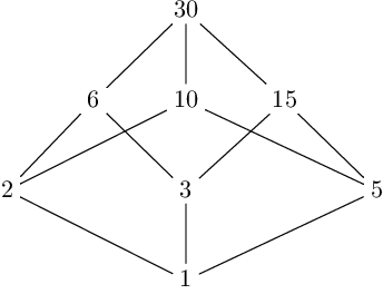
The signs of the w_{d^{\prime}} remain to be determined. To be able to visualize them we use the Hasse diagram, by which all the divisors of a given number can be represented, in this case P(z) = 30:

Figure 1: The Hasse diagram of the number 30

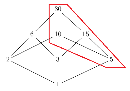
The indices d^{\prime} of the w_{d^{\prime}}s to add/subtract to obtain \lambda_d correspond to all numbers reachable from d in the Hasse diagram, going upwards. For example, we saw that the formula for d = 5 is 5 \left(w_5 - w_{10} - w_{15} + w_{30} \right), and the numbers reachable from 5 going upwards are the same indices that appear in the formula:

Figure 2: the Hasse diagram of the number 30, highlighting the multiples of 5

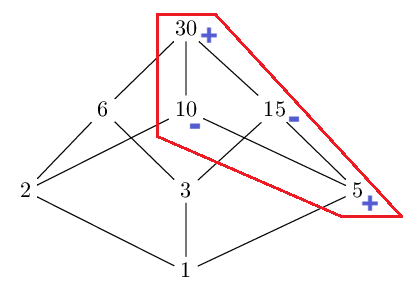
Once the w_{d^{\prime}}s have been identified, the signs are given by the following rule:

  • The sign of w_{d^{\prime}} is positive if d^{\prime} is reachable from d in an even number of steps
  • The sign of w_{d^{\prime}} is negative if d^{\prime} is reachable from d in an odd number of steps

For example, for d = 5 the signs are as follows:

Figure 3: the Hasse diagram of the number 30, highlighting the multiples of 5 with the sign they have in the dual Möbius inversion formula

Indeed:

  • 5 is reachable from 5 in 0 steps; 0 is an even number and therefore w_5 has a positive sign.
  • 10 and 15 are reachable from 5 in 1 step; 1 is an odd number and therefore w_{10} and w_{15} have a negative sign.
  • 30 is reachable from 5 in 2 steps; 2 is an even number and therefore w_{30} has a positive sign. We observe that 30 can be reached from 5 via two different paths but both composed of two steps, so the sign does not depend on the path considered; this is a general property of Hasse diagrams that allows the calculation of the sign to be unambiguous.

In general the following formula applies:

\lambda_d = d \sum_{d \mid d^{\prime} \mid 30} \mu\left(\frac{d^{\prime}}{d} \right) w_{d^{\prime}}

In fact \frac{d^{\prime}}{d} has as many distinct prime factors as the number of steps that separate d and d^{\prime} in the Hasse diagram (since each step corresponds to multiplication by a different prime factor); furthermore the function \mu returns 1 if this number is even, -1 if it’s odd.

Starting from the example and using the generic P(z) instead of 30, we’ll obtain the formula:

\lambda_d = d \sum_{d \mid d^{\prime} \mid P(z)} \mu\left(\frac{d ^{\prime}}{d} \right) w_{d^{\prime}} \tag{10}

The proof is an application of a theorem called the dual Möbius inversion formula. We’ll leave the details to interested readers.

What does the dual Möbius inversion formula consist of and how is it applied to prove (10)?

Dual Möbius inversion formula

Let n be a positive natural number and let f be a function defined on the divisors of n.
Let g be the following function defined on the divisors of n:

g(d) := \sum_{d \mid d^{\prime} \mid n} f(d^{\prime})

Then, for each k \mid n:

f(k) = \sum_{k \mid d \mid n} \mu \left(\frac{d}{k}\right) g(d)

Before seeing the proof, let’s see an example to understand what calculations are performed:

Suppose n = 30 and k = 2. Then, by the dual Möbius inversion formula it should be:

f(2) = \sum_{2 \mid d \mid 30} \mu \left(\frac{d}{2}\right) g(d) = \sum_{2 \mid d \mid 30} \mu \left(\frac{d}{2}\right) \sum_{d \mid d^{\prime} \mid 30} f(d^{\prime}).

Let’s check that this is indeed the case:

\begin{aligned} \sum_{2 \mid d \mid 30} \mu \left(\frac{d}{2}\right) \sum_{d \mid d^{\prime} \mid 30} f(d^{\prime}) &= \\ \sum_{d \in \{2, 6, 10, 30\}} \mu \left(\frac{d}{2}\right) \sum_{d \mid d^{\prime} \mid 30} f(d^{\prime}) &= \\ \mu \left(\frac{2}{2}\right) \sum_{2 \mid d^{\prime} \mid 30} f(d^{\prime}) + \mu \left(\frac{6}{2}\right) \sum_{6 \mid d^{\prime} \mid 30} f(d^{\prime}) + \mu \left(\frac{10}{2}\right) \sum_{10 \mid d^{\prime} \mid 30} f(d^{\prime}) + \mu \left(\frac{30}{2}\right) \sum_{30 \mid d^{\prime} \mid 30} f(d^{\prime}) &= \\ \mu(1) \sum_{d^{\prime}\in\{2, 6, 10, 30\}} f(d^{\prime}) + \mu(3) \sum_{d^{\prime}\in\{6, 30\}} f(d^{\prime}) + \mu(5) \sum_{d^{\prime} \in \{10, 30\}} f(d^{\prime}) + \mu(15) \sum_{d^{\prime} \in \{30\}} f(d^{\prime}) &= \\ \left(f(2) + f(6) + f(10) + f(30)\right) - \left(f(6) + f(30) \right) - \left(f (10) + f(30) \right) + f(30) &= \text{(*)} \\ f(2) \cdot 1 + f(6) \cdot (1 - 1) + f(10) \cdot (1 - 1) + f(30) \cdot (1 - 1 - 1 + 1) &= \\ f(2) \cdot 1 + f(6) \cdot 0 + f(10) \cdot 0 + f(30) \cdot 0 &=\\ f(2) \end{aligned}.

The proof is based on the step (*) of the example: collecting the values of the function f, we can see that they are multiplied by algebraic sums which are always zero except f(k) which is always multiplied by 1; in particular, the property according to which the algebraic sums are all zero except one is Property N.11.

\begin{aligned} \sum_{k \mid d \mid n} \mu \left(\frac{d}{k}\right) \sum_{d \mid d^{\prime} \mid n} f(d^{\prime}) &= \text{[let's define $r := \frac{d}{k}$, hence $d = kr$]} \\ \sum_{kr \mid n} \mu(r) \sum_{kr \mid d^{\prime} \mid n} f(d^{\prime}) &= \text{[$kr \mid d^{\prime} \Rightarrow d^{\prime} = krs$]} \\ \sum_{kr \mid n} \mu(r) \sum_{krs \mid n} f(krs) &= \\ \sum_{r \mid \frac{n}{k}} \mu(r) \sum_{rs \mid \frac{n}{k}} f(krs) &= \\ \sum_{r \mid \frac{n}{k}} \sum_{rs \mid \frac{n}{k}} \mu(r) f(krs) &= \text{[$a := rs \Rightarrow r \mid a$]} \\ \sum_{a \mid \frac{n}{k}} \sum_{r \mid a} \mu(r) f(ka) &= \\ \sum_{a \mid \frac{n}{k}} f(ka) \sum_{r \mid a} \mu(r) &= \text{[by Property N.11, $\sum_{r \mid a} \mu(r) \neq 0 \Leftrightarrow a = 1$]} \\ f(k)\end{aligned}

In our case we must apply the dual Möbius inversion formula by setting:

  • n := P(z)
  • f(d^{\prime}) = \frac{\lambda_{d^{\prime}}}{d^{\prime}}

Hence g(d) = \sum_{d \mid d^{\prime} \mid n} f(d^{\prime}) = \sum_{d \mid d^{\prime} \mid P(z)} \frac{\lambda_{d^{\prime}}}{d^{\prime}} = w_d by (8), so we can replace w_d instead of g(d).
Let’s now start from the formula of the theorem:

f(k) = \sum_{k \mid d \mid n} \mu \left(\frac{d}{k}\right) g(d)

Making the substitutions, we’ll obtain:

\frac{\lambda_k}{k} = \sum_{k \mid d \mid P(z)} \mu \left(\frac{d}{k}\right) w_d

Multiplying by k and changing the names of the variables, we’ll obtain formula (10).

Step 7: Find the values of w_d that minimize T

This passage has more to do with algebraic calculus than with number theory, so we’ll leave it to interested readers. The important thing for the sequel is only the final result:

w_d := \frac{\mu(d)}{\phi(d) V(z)} \tag{11}

where

V(z) := \sum_{d \mid P(z)} \frac{1}{\phi(d)} \tag{12}

We can observe that, by (9), if h is any function defined on the divisors of P(z):

\sum_{d \mid P(z)} \phi(d) \left(w_d - h(d)\right)^2 = T + \sum_{d \mid P(z)} \phi(d) h(d)^2 - 2 \sum_{d \mid P(z)} \phi(d) w_d h(d)

If we set w_d := h(d), the left-hand side vanishes, so:

T = 2 \sum_{d \mid P(z)} \phi(d) w_d h(d) - \sum_{d \mid P (z)} \phi(d) h(d)^2 \tag{d}

Our aim is to find a suitable function h in order to make this value of T, obtained by substituting w_d := h(d), as small as possible.

We said that \lambda_1 must be 1, but we can also get \lambda_1 from (10). Incidentally, the reason we saw how to calculate \lambda_ds from w_ds before actually calculating w_ds is that now we need formula (10), by which:

1 = \lambda_1 = \sum_{d^{\prime} \mid P(z)} \mu\left(d^{\prime} \right) w_{d^{\prime}} = \sum_{d \mid P(z)} \mu(d) w_{d} \tag{e}

We have thus obtained a first constraint that must be satisfied by our w_ds. Comparing with (d), we can try to reduce the summation \sum_{d \mid P(z)} \phi(d) w_d h(d) to \sum_{d \mid P(z)} \mu(d) w_{d}; the simplest way to do this is to set h(d) := \frac{\mu(d)}{\phi(d)}. Let’s try to put this value into (d):

\begin{aligned} T &= \\ 2 \sum_{d \mid P(z)} \phi(d) w_d \frac{\mu(d)}{\phi(d)} - \sum_{d \mid P(z)} \phi(d) \left(\frac{\mu(d)}{\phi(d)}\right)^2 &= \\ 2 \sum_{d \mid P(z)} \mu(d) w_d - \sum_{d \mid P(z)} \frac{\mu(d)^2}{\phi(d)} &= \\ 2 - \sum_{d \mid P(z)} \frac{1}{\phi(d)} \end{aligned}

where in the last step we applied (e), furthermore we observed that \mu(d)^2 = 1 because \mu(d) = \pm 1, being d square free.
The value of T that we found is not good because for z \to +\infty it tends to -\infty, while clearly the quantity to estimate (the numbers that remain after the sieve) is positive.
To solve the problem we’ll call V(z) the last summation obtained and, instead of setting h(d) := \frac{\mu(d)}{\phi(d)} as before, we’ll divide by V(z) obtaining h(d) := \frac{\mu(d)}{\phi(d) V(z)}. Substituting this value into (d), with few changes compared to the steps seen before, we’ll obtain:

\begin{aligned} T &= \\ 2 \sum_{d \mid P(z)} \phi(d) w_d \frac{\mu(d)}{\phi(d) V(z)} - \sum_{d \mid P(z)} \phi(d) \left(\frac{\mu(d)}{\phi(d) V(z)}\right)^2 &= \\ \frac{2}{V(z)} \sum_{d \mid P(z)} \mu(d) w_d - \frac{1}{V(z)^2} \sum_{d \mid P(z)} \frac{\mu(d)^2}{\phi(d)} &= \\ \frac{2}{V(z)} - \frac{1}{V(z)^2} \sum_{d \mid P(z)} \frac{1}{\phi(d)} &= \\ \frac{2}{V(z)} - \frac{1}{V(z)^2} V(z) &= \\ \frac{2}{V(z)} - \frac{1}{V(z)} &= \\ \frac{1}{V(z)} \end{aligned}

This value of T is satisfactory because it is positive. We do not exclude that other choices of w_d could generate even smaller T values, but Selberg’s sieve makes this choice, and we invite our readers to let us know if there are better choices (i.e. that minimize T without however increasing too much the error term R, which we’ll study in the next article).

Final example

Let’s calculate T and the various \lambda_ds when P(z) = 2 \cdot 3 \cdot 5 = 30.

After various simplifications, we have seen that T can be expressed in the form of formula (9):

\begin{aligned} T & = \sum_{d \mid P(z)} \phi(d) w_d^2 \\ & = \sum_{d \mid 30} \phi(d) w_d^2 \\ & = \phi(1) w_1^2 + \phi(2) w_2^2 + \phi(3) w_3^2 + \phi(5) w_5^2 + \phi(6) w_6^2 + \phi(10) w_{10}^2 + \phi(15) w_{15}^2 + \phi(30) w_{30}^2 \\ & = w_1^2 + w_2^2 + 2 w_3^2 + 4 w_5^2 + 2 w_6^2 + 4 w_{10}^2 + 8 w_{15}^2 + 8 w_{30}^2 \end{aligned}

where in the last step we replaced the values of the \phi function calculated in the example of step 2.

Now we’ll calculate V(z), given by formula (12):

\begin{aligned} V(z) & = \sum_{d \mid P(z)} \frac{1}{\phi(d)} \\ & = \frac{1}{\phi(1)} + \frac{1}{\phi(2)} + \frac{1}{\phi(3)} + \frac{1}{\phi(5)} + \frac{1}{\phi(6)} + \frac{1}{\phi(10)} + \frac{1}{\phi(15)} + \frac{1}{\phi(30)} \\ & = \frac{1}{1} + \frac{1}{1} + \frac{1}{2} + \frac{1}{4} + \frac{1}{2} + \frac{1}{4} + \frac{1}{8} + \frac{1}{8} \\ & = \frac{15}{4} \end{aligned}

We can thus calculate the values of w_d, given by (10):

\begin{aligned} w_1 & = \frac{\mu(1)}{\phi(1) V(z)} = \frac{1}{1 \cdot \frac{15}{4}} = \frac{4}{15} \\ w_2 & = \frac{\mu(2)}{\phi(2) V(z)} = \frac{-1}{1 \cdot \frac{15}{4}} = - \frac{4}{15} \\ w_3 & = \frac{\mu(3)}{\phi(3) V (z)} = \frac{-1}{2 \cdot \frac{15}{4}} = - \frac{2}{15} \\ w_5 & = \frac{\mu(5)}{\phi(5) V(z)} = \frac{-1}{4 \cdot \frac{15}{4}} = - \frac{1}{15} \\ w_6 & = \frac{\mu(6)}{\phi(6) V(z)} = \frac{1}{2 \cdot \frac{15}{4}} = \frac{2}{15} \\ w_{10} & = \frac{\mu(10)}{\phi(10) V(z)} = \frac{1}{4 \cdot \frac{15}{4}} = \frac{1}{15} \\ w_{15} & = \frac{\mu(15)}{\phi(15) V(z)} = \frac{1}{8 \cdot \frac{15}{4}} = \frac{1}{30} \\ w_{30} & = \frac{\mu(30)}{\phi(30) V(z)} = \frac{-1}{8 \cdot \frac{15}{4}} = -\frac{1}{30} \end{aligned}

Substituting T into the formula, we’ll have:

\begin{aligned} T & = w_1^2 + w_2^2 + 2 w_3^2 + 4 w_5^2 + 2 w_6^2 + 4 w_{10}^2 + 8 w_{15}^2 + 8 w_{30}^2 \\ & = \left(\frac{4}{15} \right)^2 + \left(-\frac{4}{15} \right)^2 + 2 \left(-\frac{2}{15} \right)^2 + 4 \left(-\frac{1}{15} \right)^2 + 2 \left(\frac{2}{15} \right)^2 + 4 \left(\frac{1}{15} \right)^2 + 8 \left(\frac{1}{30} \right) ^2 + 8 \left(-\frac{1}{30} \right)^2 \\ & = \frac{4}{15} \end{aligned}

So we can say that, according to Selberg’s sieve, the number of elements of the set A that remain after eliminating the multiples of 2, those of 3 and those of 5, is approximately \frac{4}{15} of the total (without taking into account the error term).

To conclude, we’ll calculate the values of \lambda_d using formula (10).

First let’s check that \lambda_1 = 1:

\begin{aligned} \lambda_1 &= \\ 1 \sum_{1 \mid d^{\prime} \mid 30} \mu\left(\frac{d^{\prime}}{1} \right) w_{d^{\prime}} &= \\ \sum_{d^{\prime} \in \{1, 2, 3, 5, 6, 10, 15, 30\}} \mu\left(\frac{d^{\prime}}{1} \right) w_{d^{\prime}} &= \\ \mu\left(\frac{1}{1} \right) w_{1} + \mu\left(\frac{2}{1} \right) w_{2} + \mu\left(\frac{3}{1} \right) w_{3} + \mu\left(\frac{5}{1} \right) w_{5} + \\ \mu\left(\frac{6}{1} \right) w_{6} + \mu\left(\frac{10}{1} \right) w_{10} + \mu\left(\frac{15}{1} \right) w_{15} + \mu\left(\frac{30}{1} \right) w_{30} &= \\ w_1 - w_2 - w_3 - w_5 + w_6 + w_{10} + w_{15} - w_{30} &= \\ \frac{4}{15} - \left(- \frac{4}{15}\right) - \left(-\frac{2}{15}\right) - \left(- \frac{1}{15}\right) + \frac{2}{15} + \frac{1}{15} + \frac{1}{30} - \left(- \frac{1}{30}\right) &= \\ 1 \end{aligned}

Let’s now calculate \lambda_2:

\begin{aligned} \lambda_2 &= \\ 2 \sum_{2 \mid d^{\prime} \mid 30} \mu\left(\frac{d^{\prime}}{2} \right) w_{d^{\prime}} &= \\ 2 \sum_{d^{\prime} \in \{2, 6, 10, 30\}} \mu\left(\frac{d^{\prime}}{2} \right) w_{d^{\prime}} &= \\ 2 \left(\mu\left(\frac{2}{2} \right) w_{2} + \mu\left(\frac{6}{2} \right) w_{6} + \mu\left(\frac{10}{2} \right) w_{10} + \mu\left(\frac{30}{2} \right) w_{30} \right) &= \\ 2 \left(w_2 - w_6 - w_{10} + w_{30} \right) &= \\ 2 \left(\left(- \frac{4}{15}\right) -\frac{2}{15} - \frac{1}{15} + \left(- \frac{1}{30}\right) \right) &= \\ 2 \cdot \left(-\frac{1}{2}\right) &= \\ -1 \end{aligned}

With similar steps we can get the values of the other \lambda_ds. Here is the complete list:

\lambda_1, \lambda_2, \lambda_3, \lambda_5, \lambda_6, \lambda_{10}, \lambda_{15}, \lambda_{30} = 1, -1, -1, -1, 1, 1, 1, -1

These values will be used in the next article to overestimate the error term R given by formula (2).

The values obtained for \lambda(d) correspond, in this case, to \mu(d). We assume that this always happens for Selberg’s sieve in the simplified form, however we have not investigated why, so we invite our readers to let us know if they can find out more.

Shows the calculation details of \lambda_3, \lambda_5, \lambda_6, \lambda_{10}, \lambda_{15}, \lambda_{30}

\begin{aligned} \lambda_3 &= \\ 3 \sum_{3 \mid d^{\prime} \mid 30} \mu\left(\frac{d^{\prime}}{3} \right) w_{d^{\prime}} &= \\ 3 \sum_{d^{\prime} \in \{3, 6, 15, 30\}} \mu\left(\frac{d^{\prime}}{3} \right) w_{d^{\prime}} &= \\ 3 \left(\mu\left(\frac{3}{3} \right) w_{3} + \mu\left(\frac{6}{3} \right) w_{6} + \mu\left(\frac{15}{3} \right) w_{15} + \mu\left(\frac{30}{3} \right) w_{30} \right) &= \\ 3 \left(w_3 - w_6 - w_{15} + w_{30} \right) &= \\ 3 \left(\left(- \frac{2}{15}\right) -\frac{2}{15} - \frac{1}{30} + \left(- \frac{1}{30}\right) \right) &= \\ 3 \cdot \left(-\frac{1}{3}\right) &= \\ -1 \end{aligned}
\begin{aligned} \lambda_5 &= \\ 5 \sum_{5 \mid d^{\prime} \mid 30} \mu\left(\frac{d^{\prime}}{5} \right) w_{d^{\prime}} &= \\ 5 \sum_{d^{\prime} \in \{5, 10, 15, 30\}} \mu\left(\frac{d^{\prime}}{5} \right) w_{d^{\prime}} &= \\ 5 \left(\mu\left(\frac{5}{5} \right) w_{5} + \mu\left(\frac{10}{5} \right) w_{10} + \mu\left(\frac{15}{5} \right) w_{15} + \mu\left(\frac{30}{5} \right) w_{30} \right) &= \\ 5 \left(w_5 - w_{10} - w_{15} + w_{30} \right) &= \\ 5 \left(\left(- \frac{1}{15}\right) -\frac{1}{15} - \frac{1}{30} + \left(- \frac{1}{30}\right) \right) &= \\ 5 \cdot \left(-\frac{1}{5}\right) &= \\ -1 \end{aligned}
\begin{aligned} \lambda_6 &= \\ 6 \sum_{6 \mid d^{\prime} \mid 30} \mu\left(\frac{d^{\prime}}{6} \right) w_{d^{\prime}} &= \\ 6 \sum_{d^{\prime} \in \{6, 30\}} \mu\left(\frac{d^{\prime}}{6} \right) w_{d^{\prime}} &= \\ 6 \left(\mu\left(\frac{6}{6} \right) w_{6} + \mu\left(\frac{30}{6} \right) w_{30} \right) &= \\ 6 \left(w_6 - w_{30} \right) & = \\ 6 \left(\frac{2}{15} - \left(- \frac{1}{30}\right) \right) &= \\ 6 \cdot \left(\frac{1}{6}\right) &= \\ 1 \end{aligned}
\begin{aligned} \lambda_{10} &= \\ 10 \sum_{10 \mid d^{\prime} \mid 30} \mu\left(\frac{d^{\prime}}{10} \right) w_{d^{\prime}} &= \\ 10 \sum_{d^{\prime} \in \{10, 30 \}} \mu\left(\frac{d^{\prime}}{10} \right) w_{d^{\prime}} &= \\ 10 \left(\mu\left(\frac{10}{10} \right) w_{10} + \mu\left(\frac{30}{10} \right) w_{30} \right) &= \\ 10 \left(w_{10} - w_{30} \right) &= \\ 10 \left(\frac{1}{15} - \left(- \frac{1}{30}\right) \right) &= \\ 10 \cdot \left(\frac{1}{10}\right) &= \\ 1 \end{aligned}
\begin{aligned} \lambda_{15} &= \\ 15 \sum_{15 \mid d^{\prime} \mid 30} \mu\left(\frac{d^{\prime}}{15} \right) w_{d^{\prime}} &= \\ 15 \sum_{d^{\prime} \in \{15, 30 \}} \mu\left(\frac{d^{\prime}}{15} \right) w_{d^{\prime}} &= \\ 15 \left(\mu\left(\frac{15}{15} \right) w_{15} + \mu\left(\frac{30}{15} \right) w_{30} \right) &= \\ 15 \left(w_{15} - w_{30} \right) &= \\ 15 \left(\frac{1}{30} - \left(- \frac{1}{30}\right) \right) &= \\ 15 \cdot \left(\frac{1}{15}\right) &= \\ 1 \end{aligned}
\begin{aligned} \lambda_{30} &= \\ 30 \sum_{30 \mid d^{\prime} \mid 30} \mu\left(\frac{d^{\prime}}{30} \right) w_{d^{\prime}} &= \\ 30 \sum_{d^{\prime} \in \{30\}} \mu\left(\frac{d^{\prime}}{30} \right) w_{d^{\prime}} &= \\ 30 \mu\left(\frac{30}{30} \right) w_{30} &= \\ 30 w_{30} &= \\ 30 \left(- \frac{1}{30}\right) &= \\ -1 \end{aligned}

2 Replies to “Selberg’s sieve: study of the parameters λ”

  1. I’m glad to see that you’ve come around to the usefulness of a sieve function for proving Goldbach’s. It’s also good that you’ve searched out and found related theorems that apply. Do you still have the opinion that proof by a negative (reductio ad absurdum) is not valid? (that is, proof of Goldbach’s via sieve function).

    1. Generally speaking, we believe in sieve theory as a good candidate for proving Goldbach’s Conjecture. Unfortunately, simplistic approaches are not valid, like those based on Erathostenes’ sieve, which shows up its limits when applied to Goldbach’s Conjecture, and generally to problems which involve counting prime numbers, as we explained in the following articles: Why don’t algorithmic approaches work well in sieve theory? (part I), Why don’t algorithmic approaches work well in sieve theory? (part II). However, we think that more sophisticated sieving techniques may be successful in proving the Conjecture. Regarding a reductio ad absurdum, out attempts move mostly towards a direct proof, but… who knows?

Leave a Reply

Your email address will not be published. Required fields are marked *